Libraries for Reading Data, tibbles, and the tidyverse
Reading In Data
In 5210, we learned some standard library functions for reading in
data, including read.csv and read.table. We
also have a number of libraries/data formats supported by R Studio:
tibble. A re-imagining of the data frame, that keeps “what time has proven to be effective”. see https://r4ds.had.co.nz/tibbles.html
readr. Powerful library for reading and writing raw data files, csv, tsv, fixed width, delimited, and other table specifications. Rather than creating standard data frames, it creates tibbles. See https://r4ds.had.co.nz/data-import.html
haven. Includes files to read in Stata, SPSS, and SAS files, and do some data cleaning like transforming missing/empty values to NA.
readxl. Libraries for reading in blocks of data from excel files. This is what R studio uses to read xls files from the menu.
curl. Load web pages, including web-hosted data files.
zip/unzip. Functions in the core
utilspackage that read and write zip files. Note: on windows, “Relies on a zip program (for example that from Rtools) being in the path”.gdata. A data manipulation library. Includes time/date handling, xls file handling, and a number of data reorganization/filtering functions, that are probably replaced by dplyr and reshape and similar tidyverse libraries. I discuss some of these in the optional section below.
webreadr. Built on readr, it reads in various computer log files like access logs for web servers.
prepdat. A special-purpose data reading library focused on problems in psychology, where you process response times and accuracies, and have multiple participants with data saved in separate files. This will read in and merge multiple files, and also has response time outlier removal procedures.
In the ‘other packages’ section below, I cover the gdata package, which is fairly well replaced by haven/readxls and the like; along with prepdat; a special-purpose library that combines many different data files.
Using readr and tibbles
If you use the readr data libraries instead of the base R data reading libraries, it creates a new type of data structure called a ‘tibble’. A tibble is a data frame that generally works a bit better. Some of the advantages of a tibble are that it (usually) works as a drop-in replacement for data frames, it prints out more information when you view it, but only 5-10 rows and not all variables. It will hopefully prevent you from printing out markdown files that are 100s of pages long because a single print function is hidden somewhere in your code. They also are a bit stricter, which can avoid some errors that are hard to track down. For example, if you try to access a variable name in a data frame but it does not exist, it will return an empty data vector with the NA value. In contrast, a tibble will return an error. Finally, subsetting a column returns another tibble, whereas something like x[,1] will return a vector.
The authors suggest that reading in data into a tibble can be a lot faster as well. Tibble also better support subsetting via pipes, which is an advanced syntax that some people feel is more powerful.
Storing data in a tibble is usually seamless, but there are sometimes packages out there that will fail when given a tibble when they expect a data frame. So be on the lookout for that.
library(tibble)
library(readr)

dat1 <- read_csv("bigfive.csv")

## NOTICE THE DIFFERENCE HERE:
iris[,1]
[1] 5.1 4.9 4.7 4.6 5.0 5.4 4.6 5.0 4.4 4.9 5.4 4.8 4.8 4.3 5.8 5.7 5.4 5.1 5.7
[20] 5.1 5.4 5.1 4.6 5.1 4.8 5.0 5.0 5.2 5.2 4.7 4.8 5.4 5.2 5.5 4.9 5.0 5.5 4.9
[39] 4.4 5.1 5.0 4.5 4.4 5.0 5.1 4.8 5.1 4.6 5.3 5.0 7.0 6.4 6.9 5.5 6.5 5.7 6.3
[58] 4.9 6.6 5.2 5.0 5.9 6.0 6.1 5.6 6.7 5.6 5.8 6.2 5.6 5.9 6.1 6.3 6.1 6.4
[ reached getOption("max.print") -- omitted 75 entries ]as_tibble(iris)[,1]# A tibble: 150 × 1
Sepal.Length
<dbl>
1 5.1
2 4.9
3 4.7
4 4.6
5 5
6 5.4
7 4.6
8 5
9 4.4
10 4.9
# … with 140 more rowsUsing readxl
The gdata library (below) used to be a common way to read in excel files with read.xls function, but it uses a third-party system in perl. readxl has replaced it and I use it extensively to access others excel files. It can be fussy to specify files, pages, and ranges of cells, but it seems to work really well.
#head(data)
library(readxl)
data2 <- read_excel("bigfive-codingcomplete.xlsx")

## do the same thing with gdata read.xls
#data <- read.xls("bigfive-codingcomplete.xlsx")
The tibble library imports a function called glimpse, which is like a transposed print. It can be helpful looking at large data sets read in from strange files:
library(tibble)
#library(formatR)
glimpse(data2)
Rows: 1,017
Columns: 53
$ Subnum <dbl> 1, 2, 3, 4, 5, 6, 7, 8, 9, 10, 11, 12, 13, 14, 15, 16, 17,…
$ Gender <chr> "F", "M", "F", "M", "M", "F", "F", "M", "F", "F", "F", "F"…
$ Education <dbl> 2, 2, 3, 3, 1, 2, 3, 3, 1, 3, 3, 1, 2, 2, 2, 1, 3, 2, 1, 3…
$ Q1 <dbl> 3, 4, 2, 3, 2, 5, 4, 1, 4, 4, 3, 2, 3, 2, 2, 4, 3, 4, 5, 3…
$ Q2 <dbl> 4, 4, 2, 3, 4, 2, 3, 4, 4, 2, 3, 3, 2, 2, 2, 3, 3, 5, 4, 4…
$ Q3 <dbl> 4, 3, 5, 4, 4, 4, 5, 4, 4, 5, 5, 5, 4, 3, 4, 4, 3, 4, 4, 3…
$ Q4 <dbl> 2, 2, 1, 4, 4, 1, 3, 4, 3, 2, 4, 2, 1, 4, 2, 2, 3, 2, 3, 5…
$ Q5 <dbl> 3, 3, 3, 2, 4, 3, 1, 2, 3, 4, 2, 4, 4, 5, 2, 3, 4, 4, 4, 5…
$ Q6 <dbl> 4, 3, 4, 4, 5, 3, 3, 5, 3, 2, 2, 4, 3, 4, 3, 2, 4, 3, 2, 4…
$ Q7 <dbl> 5, 3, 4, 5, 3, 4, 4, 3, 3, 4, 4, 4, 4, 3, 4, 4, 4, 3, 5, 4…
$ Q8 <dbl> 4, 4, 4, 2, 2, 4, 4, 4, 2, 2, 2, 3, 2, 4, 2, 3, 4, 2, 3, 5…
$ Q9 <dbl> 5, 3, 5, 4, 1, 2, 4, 4, 3, 4, 4, 3, 4, 1, 3, 2, 2, 3, 3, 4…
$ Q10 <dbl> 5, 5, 3, 4, 4, 4, 5, 5, 4, 5, 4, 5, 5, 5, 4, 5, 3, 4, 3, 5…
$ Q11 <dbl> 3, 3, 2, 1, 1, 4, 5, 3, 3, 5, 2, 3, 4, 5, 3, 4, 3, 4, 3, 2…
$ Q12 <dbl> 2, 3, 2, 2, 2, 2, 2, 4, 4, 1, 1, 1, 2, 2, 1, 1, 1, 1, 1, 1…
$ Q13 <dbl> 2, 5, 5, 4, 4, NA, 4, 5, 4, 4, 5, 5, 4, 3, 5, 5, 2, 4, 4, …
$ Q14 <dbl> 4, 5, 1, 2, 4, 3, 4, 4, 4, 3, 5, 3, 3, 4, 3, 4, 4, 5, 3, 4…
$ Q15 <dbl> 4, 3, 2, 2, 4, 4, 4, 5, 4, 2, 3, 5, 3, 5, 3, 3, 3, 4, 5, 5…
$ Q16 <dbl> 2, 4, 1, 4, 2, 4, 3, 2, 3, 4, 3, 3, 3, 5, 3, 5, 5, 3, 4, 4…
$ Q17 <dbl> 5, 3, 3, 5, 2, 4, 5, 3, 2, 4, 5, 5, 4, 4, 4, 3, 5, 4, 5, 5…
$ Q18 <dbl> 4, 1, 3, 4, 5, 2, 1, 4, 1, 2, 5, 2, 1, 5, 1, 3, 4, 1, 4, 5…
$ Q19 <dbl> 1, 5, 1, 4, 5, 3, 5, 1, 5, 2, 5, 4, 3, 5, 2, 3, 4, 5, 3, 3…
$ Q20 <dbl> 4, 4, 4, 3, 5, 3, 2, 4, 4, 4, 5, 5, 4, 5, 2, 4, 1, 4, 3, 5…
$ Q21 <dbl> 2, 4, 4, 4, 4, 1, 2, 5, 4, 2, 3, 5, 3, 4, 4, 2, 5, 3, 2, 4…
$ Q22 <dbl> 5, 4, 4, 5, 1, 5, 5, 2, 4, 1, 5, 4, 4, 1, 4, 5, 4, 4, 4, 5…
$ Q23 <dbl> 3, 5, 2, 4, 4, 4, 1, 2, 4, 2, 4, 1, 2, 3, 3, 3, 4, 2, 3, 4…
$ Q24 <dbl> 5, 3, 5, 4, 2, 3, 4, 3, 2, 4, 5, 4, 4, 1, 3, 2, 1, 4, 3, 3…
$ Q25 <dbl> 4, 3, 2, 2, 4, 3, 3, 2, 3, 5, 3, 5, 4, 5, 2, 3, 2, 3, 4, 5…
$ Q26 <dbl> 4, 5, 2, 1, 1, 4, 2, 4, 4, 4, 1, 1, 3, 2, 3, 4, 3, 5, 5, 4…
$ Q27 <dbl> 4, 5, 3, 3, 5, 3, 2, 3, 4, 1, 2, 5, 3, 5, 3, 4, 4, 4, 5, 2…
$ Q28 <dbl> 3, 4, 4, 2, 3, 3, 2, 4, 5, 4, 2, 4, 2, 1, 4, 4, 5, 2, 2, 5…
$ Q29 <dbl> 4, 3, 4, 4, 2, 3, 5, 5, 4, 4, 5, 5, 3, 3, 3, 4, 4, 3, 4, 3…
$ Q30 <dbl> 2, 4, 1, 4, 4, 4, 1, 4, 5, 2, 3, 3, 3, 4, 4, 3, 5, 5, 4, 4…
$ Q31 <dbl> 5, 4, 2, 4, 5, 4, 2, 3, 5, 2, 1, 5, 4, 5, 4, 5, 3, 3, 4, 2…
$ Q32 <dbl> 3, 5, 3, 4, 4, 3, 4, 4, 4, 2, 4, 4, 4, 5, 4, 2, 5, 3, 2, 4…
$ Q33 <dbl> 5, 5, 4, 5, 4, 4, 5, 2, 4, 4, 5, 4, 4, 4, 4, 5, 4, 4, 5, 5…
$ Q34 <dbl> 4, 5, 3, 3, 3, 4, 5, 5, 3, 5, 4, 5, 4, 2, 3, 4, 2, 4, 5, 3…
$ Q35 <dbl> 5, 4, 5, 4, 2, 4, 4, 4, 4, 4, 5, 4, 3, 3, 4, 4, 5, 4, 4, 5…
$ Q36 <dbl> 3, 5, 4, 3, 2, 3, 4, 5, 5, 3, 5, 1, 2, 2, 4, 3, 5, 3, 4, 2…
$ Q37 <dbl> 3, 5, 2, 2, 1, 5, 2, 2, 4, 5, 3, 2, 4, 1, 3, 5, 2, 4, 5, 2…
$ Q38 <dbl> 2, 4, 3, 2, 3, 3, 2, 4, 4, 2, 2, 2, 2, 2, 2, 3, 4, 4, 1, 2…
$ Q39 <dbl> 3, 4, 2, 3, 4, NA, 5, 5, 3, 4, 4, 5, 4, 3, 3, 4, 4, 4, 4, …
$ Q40 <dbl> 1, 4, 1, 3, 5, 3, 3, 3, 4, 2, 5, 4, 4, 5, 3, 2, 2, 2, 3, 1…
$ Q41 <dbl> 4, 3, NA, 4, 4, 4, 4, 3, 4, 4, 5, 5, 4, 5, 3, 5, 4, 4, 4, …
$ Q42 <dbl> 2, 5, 5, 4, 1, 2, 5, 2, 3, 4, 5, 1, 2, 1, 2, 2, 2, 3, 4, 4…
$ Q43 <dbl> 4, 4, 2, 4, 2, 4, 3, 4, 3, 4, 3, 3, 4, 4, 4, 5, 4, 3, 4, 2…
$ Q44 <dbl> 4, 5, 4, 4, 4, 4, 5, 3, 3, 2, 2, 4, 3, 5, 4, 3, 5, 2, 4, 4…
$ Extra <dbl> 2.750, 3.500, 2.375, 2.250, 1.500, 3.750, 3.625, 2.500, 3.…
$ Agreeable <dbl> 3.444444, 3.111111, 3.888889, 4.111111, 2.888889, 3.111111…
$ Consc <dbl> 2.777778, 3.444444, 3.777778, 3.000000, 3.222222, 3.000000…
$ Neuro <dbl> 2.250000, 3.250000, 1.750000, 3.000000, 3.875000, 2.714286…
$ Openness <dbl> 3.0, 3.6, 2.7, 2.8, 4.0, 3.2, 2.8, 3.3, 3.4, 3.0, 2.9, 3.8…
$ extrabinary <chr> "I", "E", "I", "I", "I", "E", "E", "I", "I", "E", "E", "I"…print(data2)# A tibble: 1,017 × 53
Subnum Gender Education Q1 Q2 Q3 Q4 Q5 Q6 Q7 Q8 Q9
<dbl> <chr> <dbl> <dbl> <dbl> <dbl> <dbl> <dbl> <dbl> <dbl> <dbl> <dbl>
1 1 F 2 3 4 4 2 3 4 5 4 5
2 2 M 2 4 4 3 2 3 3 3 4 3
3 3 F 3 2 2 5 1 3 4 4 4 5
4 4 M 3 3 3 4 4 2 4 5 2 4
5 5 M 1 2 4 4 4 4 5 3 2 1
6 6 F 2 5 2 4 1 3 3 4 4 2
7 7 F 3 4 3 5 3 1 3 4 4 4
8 8 M 3 1 4 4 4 2 5 3 4 4
9 9 F 1 4 4 4 3 3 3 3 2 3
10 10 F 3 4 2 5 2 4 2 4 2 4
# … with 1,007 more rows, and 41 more variables: Q10 <dbl>, Q11 <dbl>,
# Q12 <dbl>, Q13 <dbl>, Q14 <dbl>, Q15 <dbl>, Q16 <dbl>, Q17 <dbl>,
# Q18 <dbl>, Q19 <dbl>, Q20 <dbl>, Q21 <dbl>, Q22 <dbl>, Q23 <dbl>,
# Q24 <dbl>, Q25 <dbl>, Q26 <dbl>, Q27 <dbl>, Q28 <dbl>, Q29 <dbl>,
# Q30 <dbl>, Q31 <dbl>, Q32 <dbl>, Q33 <dbl>, Q34 <dbl>, Q35 <dbl>,
# Q36 <dbl>, Q37 <dbl>, Q38 <dbl>, Q39 <dbl>, Q40 <dbl>, Q41 <dbl>,
# Q42 <dbl>, Q43 <dbl>, Q44 <dbl>, Extra <dbl>, Agreeable <dbl>, …There are sometimes multiple sheets in a spreadsheet. By default this will grab the first sheet. A specific sheet can be specified too. This reads the second sheet, which is just the composite (mean) scores on five personality dimensions.
#data2 <- read.xls("bigfive-codingcomplete.xlsx",sheet=2)
#head(data2)
data2 <- read_excel("bigfive-codingcomplete.xlsx",sheet=2)
data2 <- read_excel("bigfive-codingcomplete.xlsx",sheet="subset")
The documentation warns that strings will be quoted, and you may need to play with the quote argument if you have quoted text in the spreadsheet, but this should work reasonably well for simple files.
Using curl
Curl is a widely used library and program for downloading files from the web. R provides a library that uses curl, which allows you to specify a web URL and a local file name and it will download/save the file. For example, here is an xlsx file that shows data about student health at an Australian university:
library(curl)

## This won't work!
#data3 <- read_excel("https://lo.unisa.edu.au/pluginfile.php/1020313/mod_book/chapter/106604/HLTH1025_2016.xlsx")


curl_download("https://lo.unisa.edu.au/pluginfile.php/1020313/mod_book/chapter/106604/HLTH1025_2016.xlsx",destfile="HLTH1025_2016.xlsx")

data3 <- read_excel("HLTH1025_2016.xlsx",sheet="Data")

codesheet <- read_excel("HLTH1025_2016.xlsx",sheet=1,skip=2)
You can verify that the xlsx file has been dowloaded to your working directory and look at it. Note that it has two worksheets. The first worksheet is ‘Metadata’, which is the code book for the survey. The second sheet is ‘Data’, which is the actual data table. We need to specify sheet=2 or sheet =“Data”, to get the right data sheet.
The haven library.
Haven can actually read web url directly. Here is the same data that is made available as an spss file. Notice it looks identical to the xls sheet.
library(haven)
data3.spss <- read_spss("https://lo.unisa.edu.au/pluginfile.php/1020313/mod_book/chapter/106604/HLTH1025_2016.sav")
You need to be careful when using other people’s data, especially when it is in SPSS format, because SPSS has a tradition of using a number like 999 or -999 as the code for missing data. I’ve heard claims that a depressingly-large number of high correlations reported in the literature occur because people have used 999 as missing data in two different variables, and fail to treat it as missing so it inflates correlations substantially.
If we look carefully, we can see 99s in mntlcurr and sf1, and 9999 in weight. Luckily, they did not choose to use 99 as a missing value for weight because there were legitimate values of 99 for weight. We’d hope that the spss format would save this. Haven has some functions to handle user-specified NA values, but at least for this current file it does not flag these values as missing, so we have to do it by hand. Note that almost every variable has one or more missing codes, so there will be a lot of data recoding if we want to analyze this data.
data3.spss$weight[data3.spss$weight==9999] <- NA
data3.spss$mntlcurr[data3.spss$mntlcurr==99] <- NA
data3.spss$mntlcurr[data3.spss$mntlcurr==99] <- NA
The Tidyverse
Tidyverse is a meta-library that loads and installs a bunch of other packages. These include:
tibble, which we just examinedggplot2, for fancy plottingdplyr, for data manipulationtidyr, for ‘tidying’ messy dataforcats, for dealing with factors and changing their orderpurrr, for functional programming; ways of applying functions to data.
These replace and improve on a lot of data management functions we have already used, like aggregate, apply/tapply/lapply, filtering, sorting,
There are a number of other secondary and related libraries in the tidyverse that do not get loaded. Most of these are led to Hadley Wickham and R Studio. To use, install ‘tidyverse’ and load the library, and it will install load all the dependent packages.
install.packages("tidyverse")
library(tidyverse)
Importantly, tidyverse loads ggplot2, dplyr, tidyr, and tibble.
The tidyverse encompasses new and more efficient ways of handling
data that update and augment many of the built-in methods provided by R.
In some cases, they are merely alternate functions that provide the same
output. Sometimes, they do things more efficiently or more easily. For
example, in the previous course, we learned how the []
operator could be used for selection, sorting, filtering, repetition,
and various related operations on data. The tidyverse provides
individual unique functions that do each of these functions separately.
So although each function might be easier to use, you now need to
remember a dozen different function names and how each works.
For example, we can do selection, aggregation, and plotting in a single pipeline:
data2 %>% select(Subnum,Gender, Education, Extra:Openness)  %>% mutate(Education=recode(Education, `1`="1.High school",`2`="2.College degree",`3`="3.Post-secondary degree")) %>%
  group_by(Gender, Education) %>%
  summarize (E=mean(Extra), A=mean(Agreeable), C=mean(Consc), N=mean(Neuro),O=mean(Openness)) %>%
  pivot_longer(cols=E:O) %>%
  ggplot(aes(x=Gender,group=Education,color=Education,y=value)) + geom_point() + geom_line() +facet_wrap(.~name,ncol=5) + theme_bw() + ylim(1,5)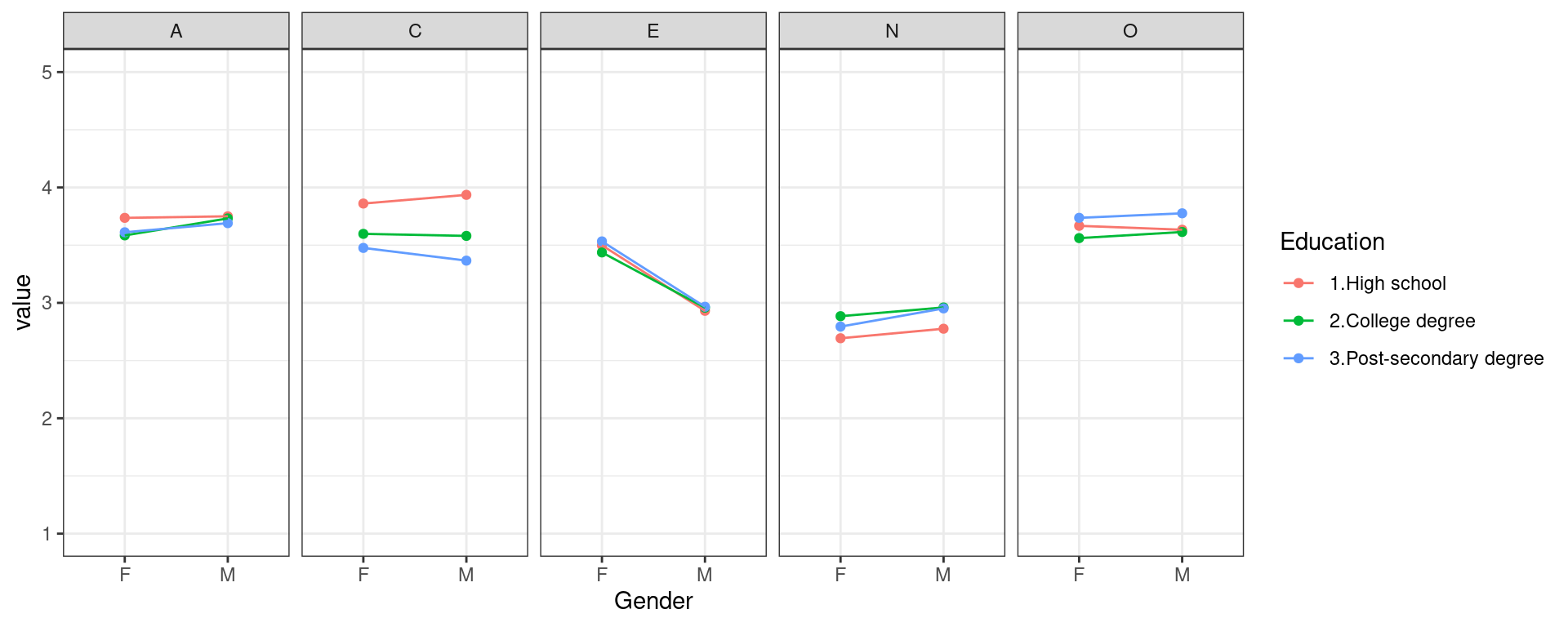
In the next units, we will learn about many of the functions supported by tidyverse libraries and functions.
Other packages
The gdata package
gdata has a lot of data management tools, related to sampling, summarizing, and the like. It has a number of useful functions for reading in .xls and .xlsx files. Note that the similar ‘’foreign’’ package includes ways of reading in additional file formats, such as spss, sas, stata, and octave, and the readxl package which is built-in to rstudio.
#install.packages("gdata")
library(gdata)
If loading the library returns an error, it is likely that you need to install perl on your computer. Instructions (courtesy Raghavendran Shankar):
Step-by-step procedure:
I have referred the cran r page : https://cran.r-project.org/web/packages/gdata/INSTALL
In the webpage, I have used the link for installing perl ( http://www.activestate.com/activeperl/) and downloaded and installed perl for 64 bit windows.
After installation, there was a folder called Perl in C drive. In that, I went to bin folder and there was an .exe file
I copied the path and used it in read.xls shown below:
data <- read.xls(“bigfive-codingcomplete”,perl = “C:/Perl64/bin/Perl.exe”)
- The data gets imported in R.
The prepdat package
The prepdat package is a new package that has two interesting functions: one that merges multiple files together, and another that aggregates summary statistics, especially useful for response time.
install.packages("prepdat")
library("prepdat")
##This might be needed on windows:
#install.packages("rtools")
utils::unzip("data.zip",exdir="data")  ##unzip the data file. This may not work on some platforms, and you may need to do it by hand.
The file_merge will merge multiple files (possibly in nested directories) with specific formats/matching strings into a single data frame:
library(prepdat)
data <- file_merge(folder_path="data", has_header=T,
                   raw_file_extension="csv",
                   raw_file_name="globallocal*")
head(data)
subnum block trial code type correctresp localstim globalstim consistency
1 105 1 1 0 0 E E O 0
2 105 1 2 0 0 E E O 0
3 105 1 3 0 0 H H O 0
4 105 1 4 0 0 E E O 0
correctLocal correctGlobal positionX positionY response correct time1 rt
1 1 NA 960 540 <rshift> 1 97295 15634
2 1 NA 960 540 <rshift> 1 114447 9514
3 1 NA 960 540 <lshift> 1 125478 1454
4 1 NA 960 540 <rshift> 1 128449 669
[ reached 'max' / getOption("max.print") -- omitted 2 rows ]There is also a ‘prep’ function that will summarize your data
data$within <- as.numeric(data$correctresp)
dat2 <- prep(dataset=data,
     dvc="rt",
     id="subnum",
     within_vars=c("within"),
     save_results=F, save_summary=T,
     results_path="data")
subnum block trial code type correctresp localstim globalstim consistency
1 105 1 1 0 0 E E O 0
2 105 1 2 0 0 E E O 0
3 105 1 3 0 0 H H O 0
4 105 1 4 0 0 E E O 0
correctLocal correctGlobal positionX positionY response correct time1 rt
1 1 NA 960 540 <rshift> 1 97295 15634
2 1 NA 960 540 <rshift> 1 114447 9514
3 1 NA 960 540 <lshift> 1 125478 1454
4 1 NA 960 540 <rshift> 1 128449 669
within
1 NA
2 NA
3 NA
4 NA
[ reached 'max' / getOption("max.print") -- omitted 2 rows ]
subnum block trial code type correctresp localstim globalstim consistency
1 105 1 1 0 0 E E O 0
2 105 1 2 0 0 E E O 0
3 105 1 3 0 0 H H O 0
correctLocal correctGlobal positionX positionY response correct time1 rt
1 1 NA 960 540 <rshift> 1 97295 15634
2 1 NA 960 540 <rshift> 1 114447 9514
3 1 NA 960 540 <lshift> 1 125478 1454
within within_condition
1 NA <NA>
2 NA <NA>
3 NA <NA>
[ reached 'max' / getOption("max.print") -- omitted 3 rows ]
subnum mdvc1 sdvc1 meddvc1 t1dvc1 t1.5dvc1 t2dvc1 n1tr1 n1.5tr1
105 105 756.2044 739.9412 650 NaN 756.2044 756.2044 0 0
106 106 515.7235 164.8607 482 NaN 515.7235 515.7235 0 0
110 110 565.1750 190.7407 535 NaN 565.1750 565.1750 0 0
n2tr1 ndvc1 p1tr1 p1.5tr1 p2tr1 rminv1 p0.05dvc1 p0.25dvc1 p0.75dvc1
105 0 680 0 0 0 641.7693 416.85 539.5 803.25
106 0 680 0 0 0 488.6712 370.95 431.0 565.00
110 0 680 0 0 0 299.7960 397.00 472.0 616.25
p0.95dvc1
105 1257.25
106 711.05
110 792.35
[ reached 'max' / getOption("max.print") -- omitted 3 rows ]