PCA, eigen decomposition and SVD

Principal Components Analysis

Principal Components Analysis (PCA) is a simple form of Factor analysis (which we will learn later). It attempts to extract latent dimensions from a set of variables. In the simplest case, suppose you have a questionnaire with 10 items on it. The first give are related to usability, and the second five are related to value. We might ask 100 people to rate a product on each of the ten dimensions. But maybe the questions on usability are all very similar, such as “How usable is the product”, “How easy is the product to use”, “How easy would it be for a novice to use the product”, etc. Similarly, suppose the value questions are also similar to one another: “Is this product a good deal?”, “Would you be willing to pay an extra 20% for this feature?”, etc. In this survey, we might expect different people to have different attitudes toward the value and usability, but they might answer all five usability questions very similarly, and all five value questions similarly, if not identically. We can simulate this as follows:

library(corrplot)
usability <- sample(1:5, 100, replace = T)
value <- sample(1:5, 100, replace = T)

qUsability <- round(usability + runif(400, min = -1, max = 1))
qValue <- round(value + runif(400, min = -1, max = 1))
qOther <- sample(0:6, 200, replace = T)

data <- matrix(c(qUsability, qValue, qOther), nrow = 100)
corrplot(cor(data))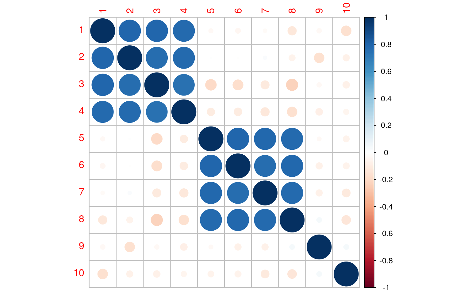

The corrplot shows that there is high positive correlation among questions 1-4 and 5-8, and two questions that look independent. This is easy to see, but if the questions were in a different order, it might not be so obvious, especially if there is a little noise:

set.seed(105)
dat2 <- data[, sample(1:10)]
corrplot(cor(dat2))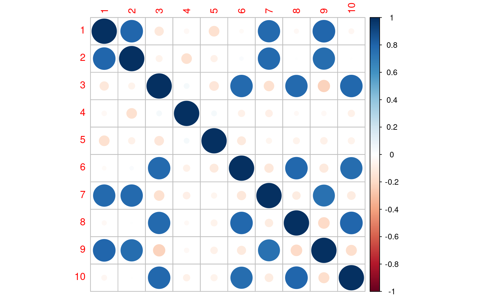

Here, we have a high-dimensional data set (10 dimensions), but really there are two major dimensions underlying these, and two minor independent dimensions. We can use eigen decomposition on the correlation matrix to find major dimensions that appear in the correlation matrix:

e <- eigen(cor(data))
plot(e$values)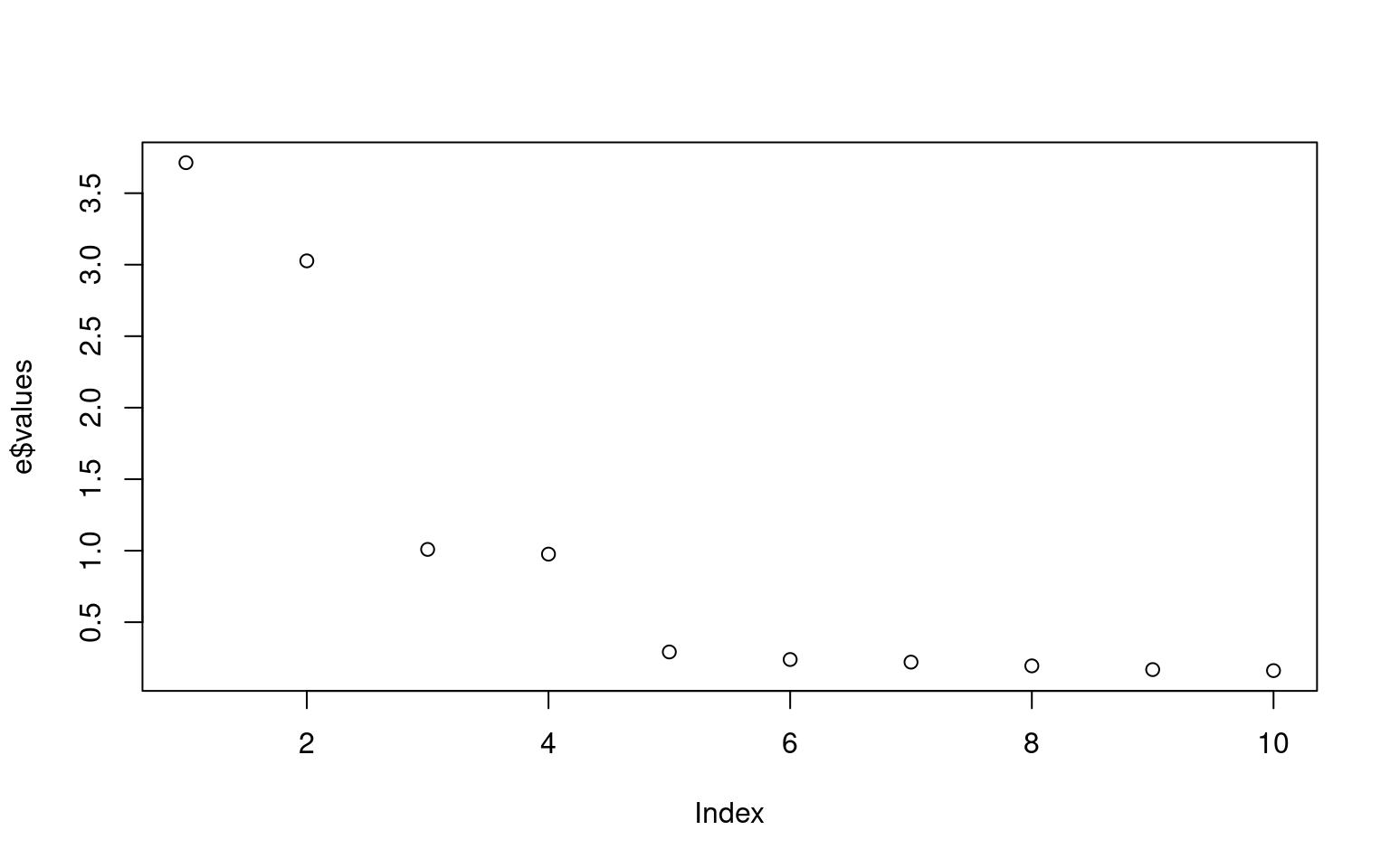

as.tibble(e$vectors) %>%
    select(V1:V4) %>%
    mutate(dimension = as.factor(1:10)) %>%
    pivot_longer(cols = 1:4) %>%
    ggplot(aes(x = dimension, y = value, group = name, fill = name)) + geom_col(position = "dodge") +
    facet_wrap(name ~ .) + theme_bw()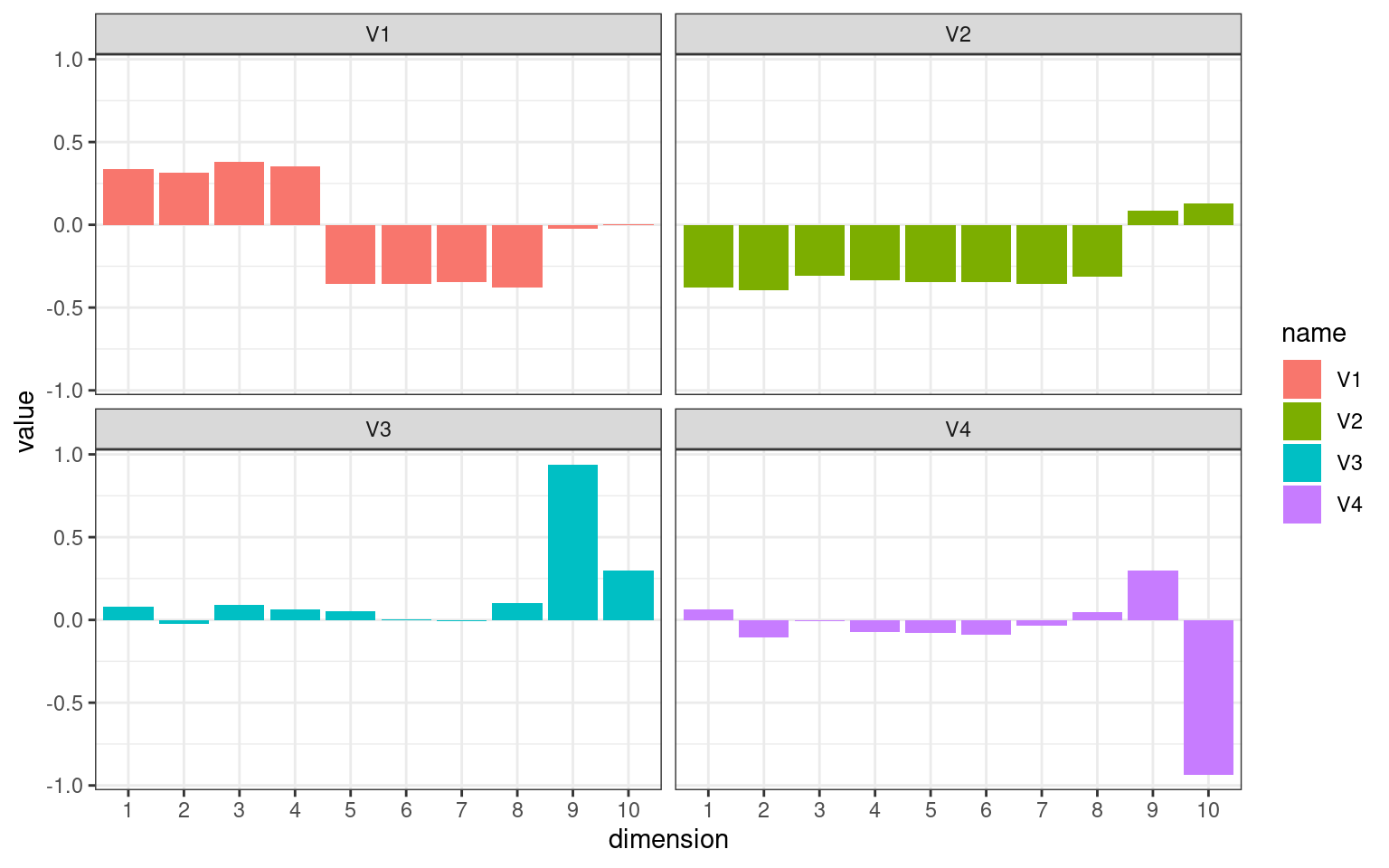

The eigen decomposition extracts a version of the sets of questions based on their inter-correlation. The eigenvectors show a degree of association of each hidden (latent) dimension with each question. Dimension V1 and V2 work together to pick out Usability and Value: V1 turns into ‘Usable and valuable’ and V2 turns into ‘difference between usable and valuable’. Similarly V3 is ‘average of Q9/Q10’ and V4 is ‘Q9-Q10’.

Eigen decomposition is otherwise known as ```Principle Components Analysis’’’ or PCA. Each vector extracted is interpreted as a principal component or hidden dimension, and the process attempts to find each dimension in order from the most to least important. Other rotations can be done as well, but we will deal with that later in the semester when we look at advances over PCA called factor analysis.

Let’s look at some simpler examples to get a better intuition for how this works.

Example: two dimensions

Suppose we had two variables we observed.

library(ggplot2)
set.seed(100)
base1 <- rnorm(20)
x1 <- base1 + rnorm(20) * 0.4
y1 <- base1 + rnorm(20) * 0.4

dat <- data.frame(id = 1:20, x1, y1)

ggplot(dat, aes(x = x1, y = y1)) + geom_point(size = 5) + geom_text(aes(label = id),
    size = 3, col = "white") + geom_abline(slope = 1, intercept = 0, linetype = 2) +
    geom_abline(slope = -1, intercept = 0, linetype = 2) + xlim(-4, 4) + ylim(-4,
    4) + theme_bw()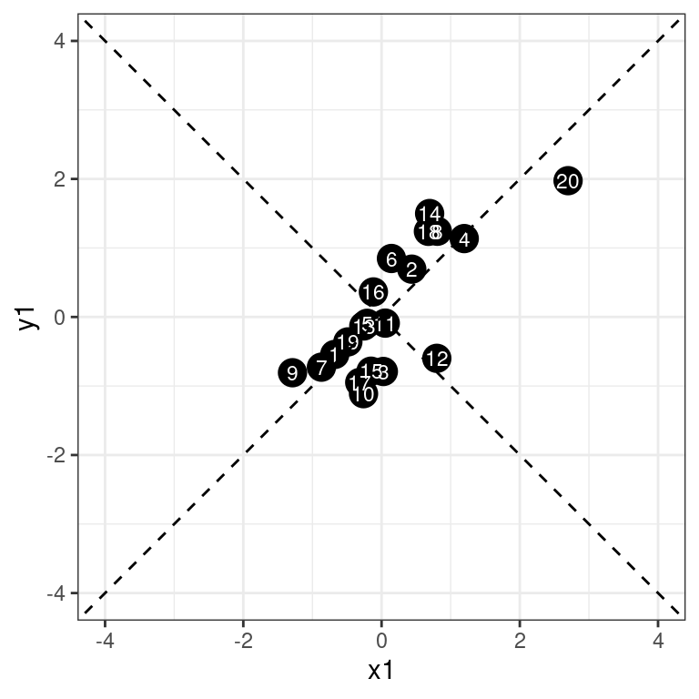

The data appear to be correlated, and falling along the line x=y. This is the vector of highest variance, and might be considered the first principal component. Since we have only two dimensions, the only remaining orthogonal dimension is the dimension along the negative diagonal–the second principal component. So, suppose we wanted to rotate the axes and redescribe the data based on these two dimensions. Any point would be re-described by its closest point on the first or second new dimension.

If we look at the the variability along this new first component, it looks like it will have a standard deviation of around 2; and the second dimension will have a standard deviation much smaller–maybe less than 1. If we do an eigen decomposition on the covariance matrix, we lose the original data (everything is filtered through the covariance matrix), but we have redescribed the data in terms of how they map onto the new vectors. The eigenvalues describe the variance of each vector–how large the dimension is.

e <- eigen(cov(dat[, -1]))
print(e)

eigen() decomposition
$values
[1] 1.4639787 0.1775083

$vectors
          [,1]       [,2]
[1,] 0.6645732 -0.7472232
[2,] 0.7472232  0.6645732

We can use the eigenvector matrix to rotate the original data into this new set of axes. Notice how the arrangement is the same with an angular rotation; all the points are in the same configuration. Also, the variance in each dimension is the same as the eigenvalues.

rotated <- data.frame(id = dat$id, as.matrix(dat[, 2:3]) %*% e$vectors)

ggplot(rotated, aes(x = X1, y = X2)) + geom_point(size = 5) + geom_text(aes(label = id),
    col = "white", size = 3) + geom_abline(intercept = 0, slope = 0) + theme_bw()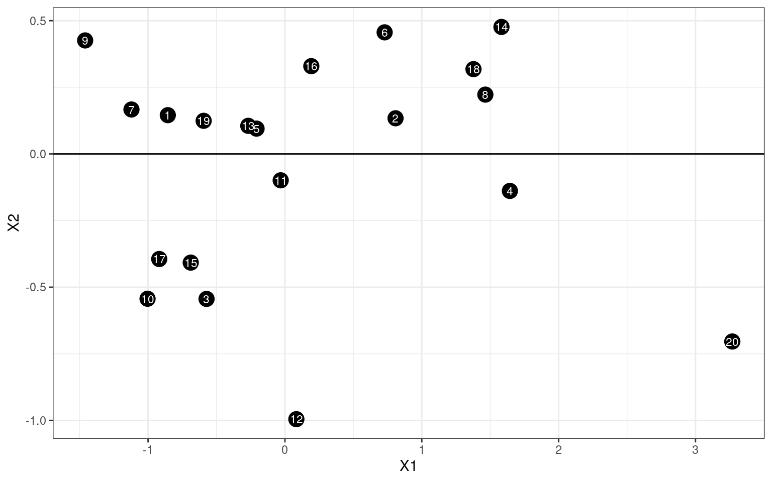

If we draw the path between points, you can probably tell that we have basically recovered the configuration but in a different orientation.

library(gridExtra)
grid.arrange(
  ggplot(dat,aes(x=x1,y=y1))+geom_point(size=5) +geom_path()+
    geom_text(aes(label=id),size=3,col="white")+
    geom_abline(slope=1,intercept=0,linetype=2) +
    geom_abline(slope=-1,intercept=0,linetype=2) +
    xlim(-3.5,3.5) + ylim(-3.5,3.5) +theme_bw(),
   
ggplot(rotated,aes(x=X1,y=X2)) + geom_point(size=5)+ geom_path()+
   geom_text(aes(label=id),col="white",size=3) + geom_abline(intercept=0,slope=0) +
  theme_bw()+ xlim(-4,4) + ylim(-4,4),
ncol=2)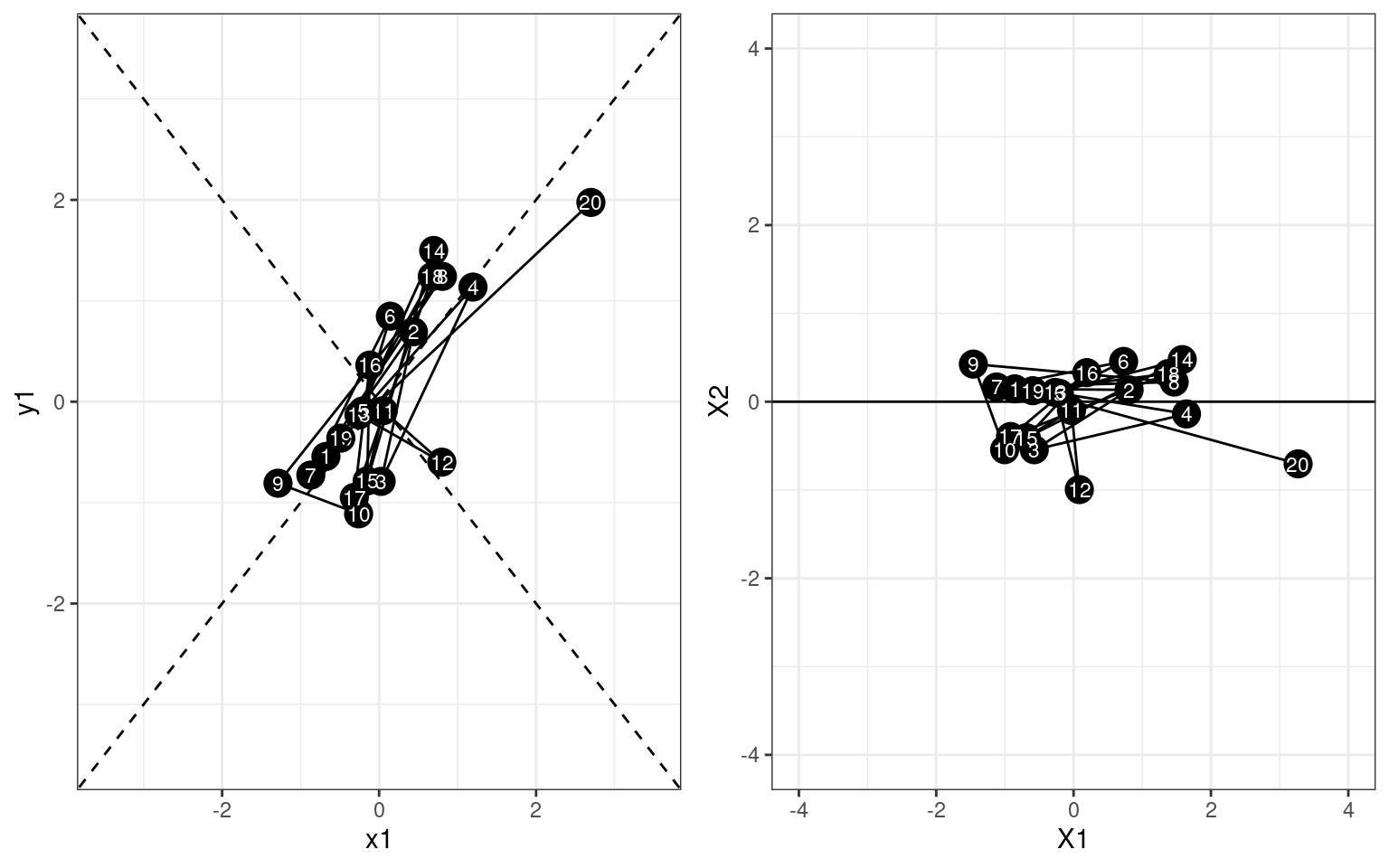

print(var(rotated$X1))

[1] 1.463979

print(var(rotated$X2))

[1] 0.1775083

So, what eigen decomposition is doing is rotating the entire space to a new set of orthogonal dimensions; so that the first axis is the one with the greatest variance, the next axis is the next-largest, and so on. In this case, because two variables were correlated, it picked the axis of greatest correlation as the first vector. If we have a lot more variables, the first most important dimension might strongly combine only some of the original values, whereas a second dimension might pick out a second set of common variance for a different set of variables.

Example of Eigen Decomposition: Two latent factors

Here is an example where there are two ‘true’ underlying factors that the data are generated from–one set of three items based on one factor, one set based on a second factor, and a final set based on both. There is noise added to each dimension, so we wouldn’t be able to compress the data into just two dimensions, but it might have most of the variance on two.

library(ggplot2)
library(GGally)

base1 <- rnorm(100)
base2 <- rnorm(100)

x1 <- base1 + rnorm(100) * 0.6
x2 <- base1 + rnorm(100) * 0.6
x3 <- base1 + rnorm(100) * 0.6

y1 <- base2 - rnorm(100) * 0.8
y2 <- base2 + rnorm(100) * 0.7
y3 <- base2 - rnorm(100) * 0.7

z1 <- (base1 + base2)/2 + rnorm(100) * 0.5
z2 <- (base1 + base2)/2 + rnorm(100) * 0.5
z3 <- (base1 + base2)/2 + rnorm(100) * 0.5

## z1 <- rnorm(100)*.5 z2 <- rnorm(100)*.5 z3 <- rnorm(100)*.5

dat <- data.frame(x1, x2, x3, y1, y2, y3, z1, z2, z3)

ggpairs(dat)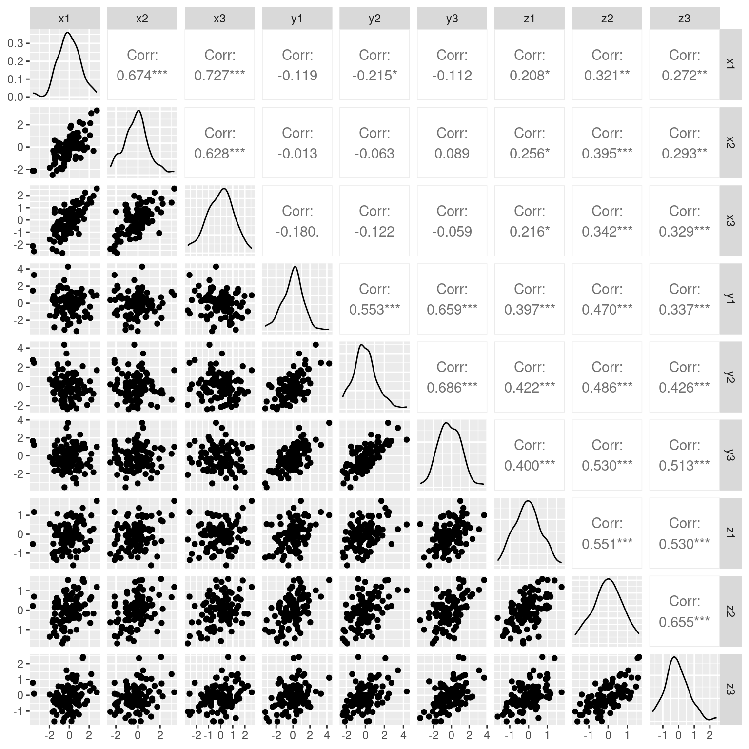

Within each set of x/y, there is moderately strong correlations; and z values are likewise correlated with everything. Rather than treating each variable separately, what if we could make a linear combination of terms–just like regression, that best combine to account for a common pool of variance. But in this case, we have two independent sources of variance. It seems like an impossible task–how can we create a regression predicting a dependent variable we don’t know? And how can we do it when the values we know are some complex unlabeled mixture of these values?

It seems remarkable, but this is what eigen decomposition does. Eigen is a german term meaning its `own’, and it is also sometimes referred to as the ‘characteristic vector’. Eigen decomposition looks at the entire multivariate set of data and finds a new set of dimensions that best characterize the shared variability of the data.

e <- eigen(cor(dat))
e$values/sum(e$values)

[1] 0.41286894 0.28711730 0.06800937 0.05967917 0.04642277 0.03897842 0.03564141
[8] 0.02732024 0.02396238

print(round(e$values, 4))

[1] 3.7158 2.5841 0.6121 0.5371 0.4178 0.3508 0.3208 0.2459 0.2157

round(e$vectors, 4)

        [,1]    [,2]    [,3]    [,4]    [,5]    [,6]    [,7]    [,8]    [,9]
 [1,] 0.1772 -0.5170  0.1414 -0.1327  0.1450 -0.2478  0.2005  0.6027  0.4217
 [2,] 0.2371 -0.4339  0.4104 -0.1334 -0.3255  0.5458 -0.2651  0.0375 -0.3062
 [3,] 0.1939 -0.4977 -0.0228  0.2182 -0.1469 -0.4068  0.3847 -0.5250 -0.2365
 [4,] 0.3227  0.3156  0.4407 -0.4484  0.3958 -0.2182  0.2012 -0.0016 -0.3953
 [5,] 0.3368  0.3371 -0.0113  0.2629 -0.6118 -0.3298 -0.0247  0.4185 -0.2116
 [6,] 0.3804  0.2831  0.3335  0.2126 -0.1054  0.3043  0.3456 -0.2642  0.5707
 [7,] 0.3779  0.0069 -0.6049 -0.6241 -0.2265  0.1285  0.1094 -0.1039  0.1060
 [8,] 0.4464 -0.0423 -0.0010  0.0826  0.2073 -0.2979 -0.7426 -0.2360  0.2308
 [ reached getOption("max.print") -- omitted 1 row ]

ggplot(data.frame(x = 1:9, values = e$values), aes(x = x, y = values)) + geom_bar(stat = "identity",
    fill = "gold", color = "grey20") + theme_bw()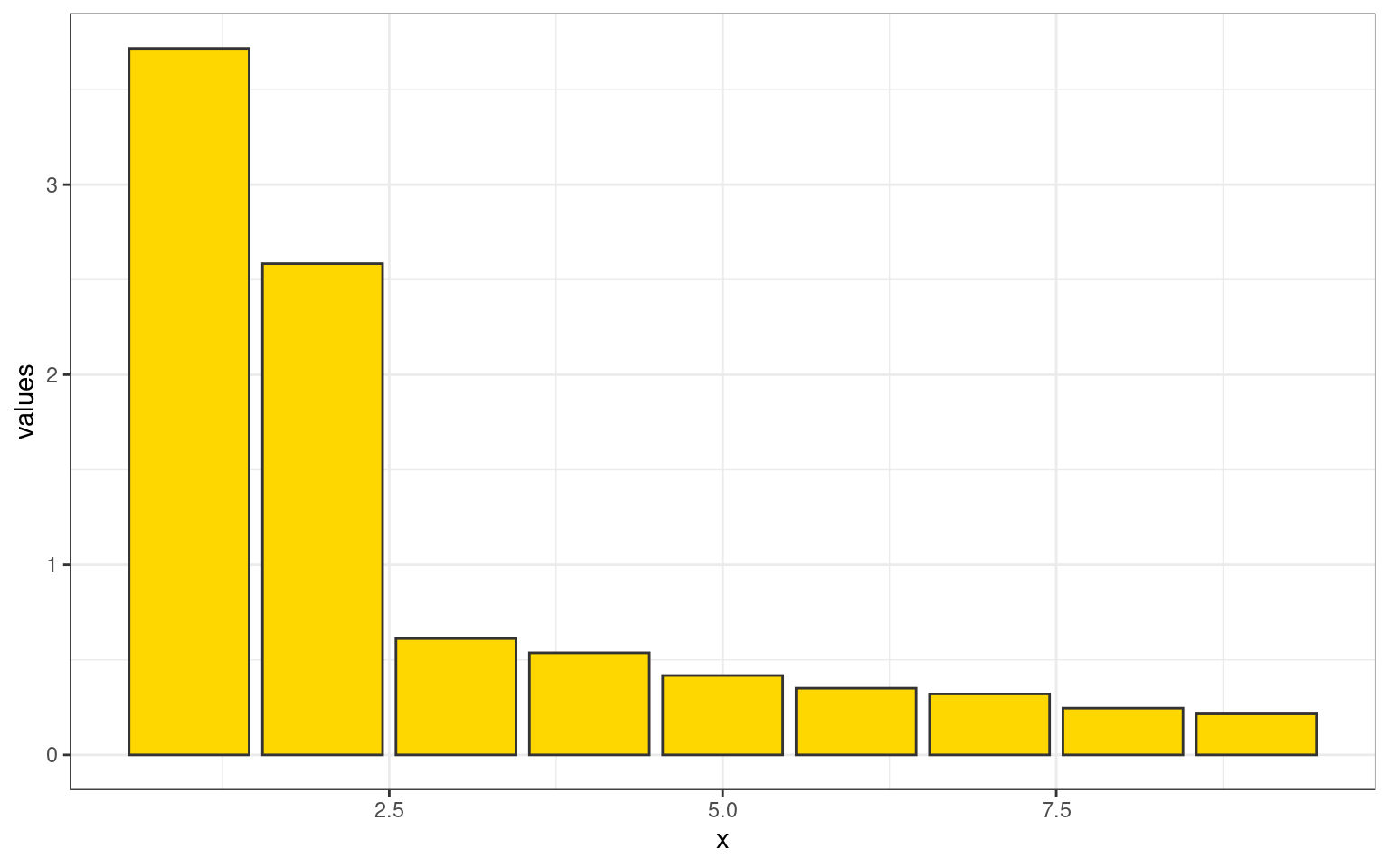

Now, the total variance in the first two dimensions is fairly large, and it trails off after that. What about the new dimensions: let’s look at just the first two dimensions:

dat <- data.frame(dim = as.factor(rep(1:9, 9)), vec = as.factor(rep(1:9, each = 9)),
    val = as.vector(e$vectors))[1:18, ]

ggplot(dat, aes(x = dim, y = val, group = vec, col = vec)) + geom_point(size = 2) +
    geom_line() + theme_bw() + scale_color_manual(values = c("gold", "black")) +
    ggtitle("Eigenvectors for first two vectors") + geom_hline(aes(yintercept = 0))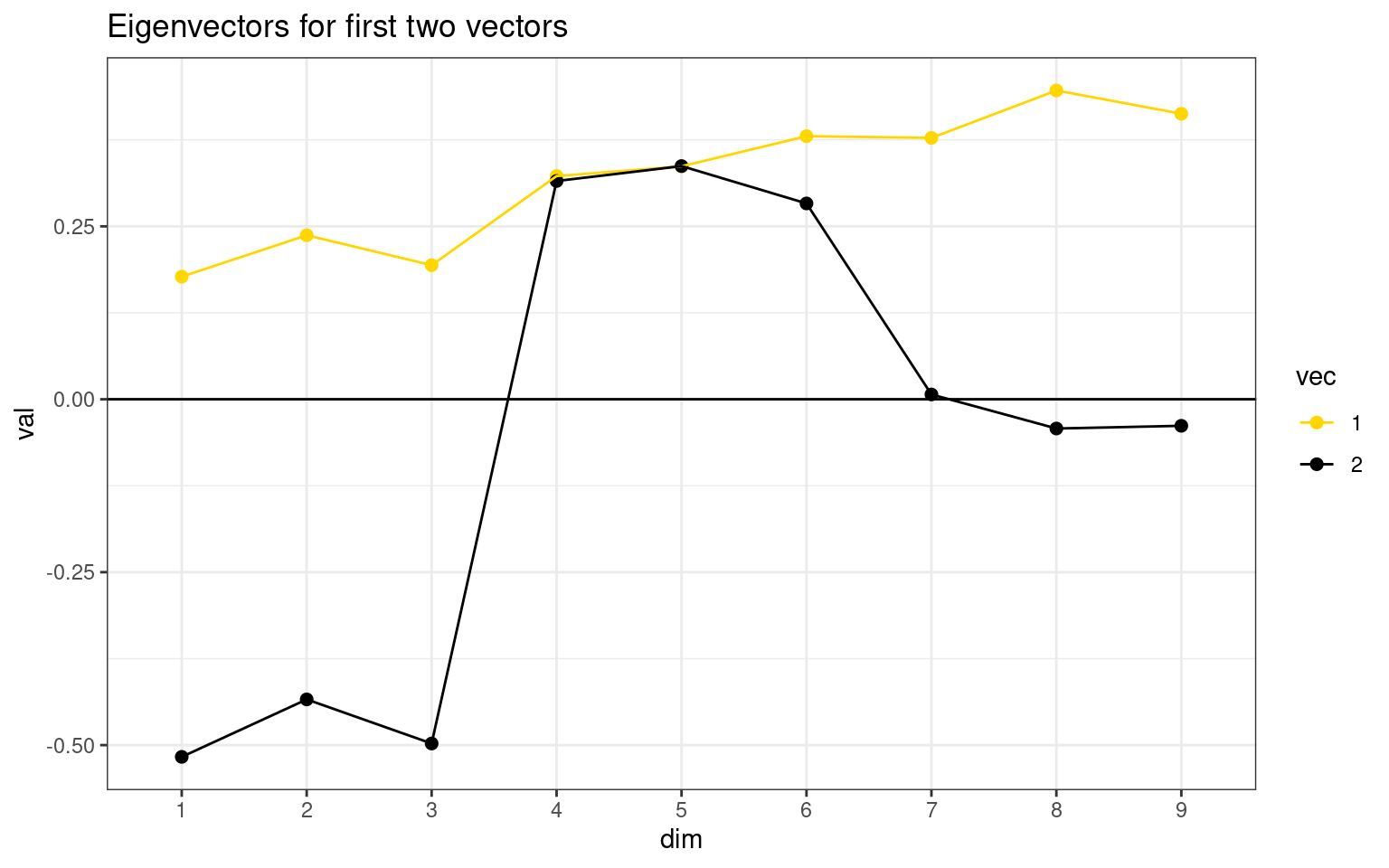

Eigenvector values are interpreted a little like correlation: positive and negative values indicate positive and negative association with the component, and values near 0 mean no association. Here, the first vector captures the shared variance across all questions–the last three questions are related to both groups. Any value close to 0 indicates that the question/item is near 0 on that component. Then, the second component gets coded as a binary factor that either explains items 1-3 or items 4-6. This sort of automatically creates a contrast coding between the first two dimensions.

Factors and Dimensions

Oftentimes, the number of things we can measure about a person are greater than the number of theoretically-interesting constructs we think these measureables explain. For example, on a personality questionairre, one asks a bunch of related questions that we believe all involve the same thing, with the hope that we will get robust and reliable measures. A person might by chance agree with one of the statements, but it is unlikely that they will agree with them all just by chance.

Measurements and questions that hang together like this are conceived of as a factor. This is similar to the previous notions of clusters, but there can be differences. A factor is a set of questions that covary together; not one in which the same answers are given by everybody. If you know all but one answer someone gives to the answers that are in a factor, you should have a pretty good idea of what the remaining answer is, regardless of whether their answer is low or high on the factor.

Thus, if you have a 10 measurements (answers) that are all a part of a common factor, and if you can project them down onto a single combined dimension without losing much information, you have a succeeded. For example, if you were to measure left arm length, right arm length, left thigh length, right thigh length, left forearm length, right forearm length, left calf length, and right calf length, chances are these will all vary fairly closely together. A factor describing these might be a weighted average of these 8 measures (maybe even weighing them all equally). These would project down from 8 dimensions to just 1 or 2. If you started adding other measurements (measurements of shoe size, weight, waist size, etc.), these may not be a closely related, and may in fact form other factors.

A number of related methods have been developed to do this sort of analysis, and they go generally under the name ‘factor analysis’, but some are also called Principal Components Analysis, exploratory factor analysis (EFA), Confirmatory Factor Analysis (CFA), and as you make more complex hypotheses about the relationship between variable, there are other related methods (Structural Equation Modeling, LISREL, MPlus, Path Analysis, etc.). The naming of these is often confusing and historically has been tied to specific software packages rather than generic analysis routines, so it is important to understand clearly what methods you are using, and what methods other are using, when you do this sort of analysis.

Typically, factor analysis focuses on analyzing the correlational structure of a set of questions or measures. When thinking about correlations, a factor might be a set of questions that are highly positively correlated within the set, but are uncorrelated with questions outside the set. Typically, negatively-correlated items are incorporated into the factor the same way positively-correlated items would be. This is somewhat like looking int the distance measures we examined with previous methods. With N questions, there are N^2 correlations in a matrix, which is sort of like placing each question is an N-dimensional space. Factor analysis attempts to find a number of dimensions smaller than N that explains most of the same data.

Example: four questions with two factors

Let’s suppose we have a set of 4 questions related to two different factors: happiness and intelligence. for example:

data <- rbind(c(5, 5.5, 100, 3), c(4.5, 5, 110, 3.5), c(3, 3.5, 130, 4), c(1, 1,
    140, 3.9), c(0, 1, 80, 2.5), c(1, 2, 90, 3.1), c(6, 6, 70, 2.3), c(2, 2.5, 60,
    1.9))
data <- data[rep(1:8, 20), ] + rnorm(640) * 0.5
# pairs(data) cor(data)
library(GGally)
ggpairs(as.data.frame(data))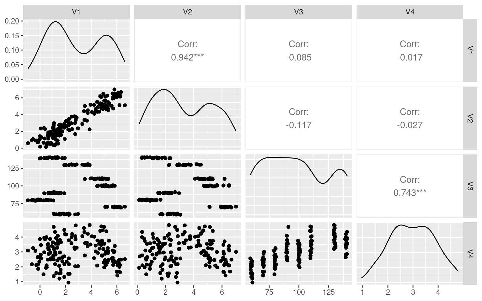

Notice that Q1/Q2 are highly correlated, as are Q3/Q4, but the there is low correlations between these clusters. A factor analysis should be able to figure it out.

When we do a PCA, we produce an outcome somewhat like an ANOVA/regression model does. That is, for an ANOVA model, you might try to predict responses based on a weighted average of predictor variables. The outcome of an eigen decomposition of the correlation matrix finds a weighted average of predictor variables that can reproduce the correlation matrix…without having the predictor variables to start with.

What PCA does is transforms the data onto a new set of axes that best account for common data.. Let’s look at the solution for two independent factors, each with two questions:

e <- eigen(cor(data))
plot(e$values)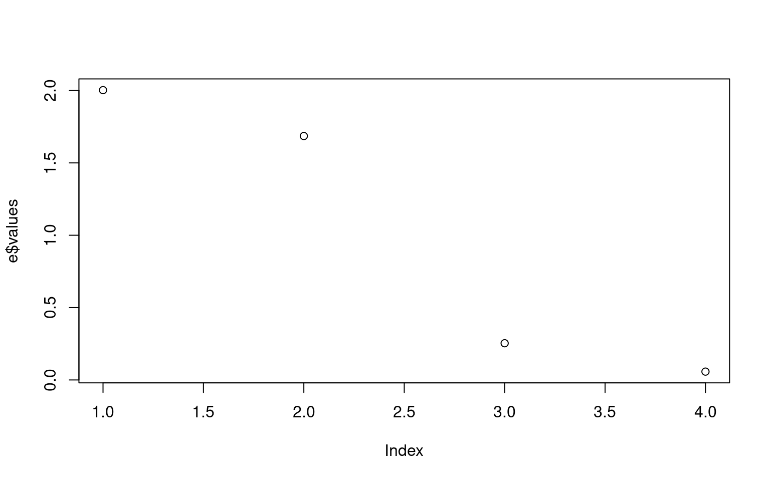

e$vectors

           [,1]       [,2]        [,3]        [,4]
[1,] -0.6354600 -0.3093395 -0.07344060  0.70363778
[2,] -0.6423071 -0.2930555  0.00702518 -0.70817425
[3,]  0.3305893 -0.6228722 -0.70734003 -0.04910223
[4,]  0.2726590 -0.6560928  0.70301295  0.03117817

barplot(t(e$vectors[, 1:2]), beside = T)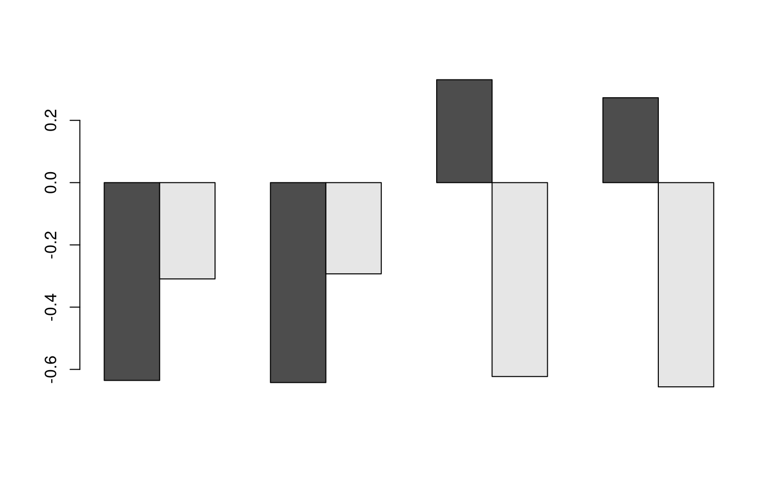

If we look at e\$values, this gives a measure of the importance of each dimension. e$vectors gives us the actual dimensions. Each column of e$vectors is considered a factor–a way of weighting answers from each question to compute a composite. Here, after 2 dimensions, the eigen values go below 1.0, and fall off considerably, indicating most of the variability is accounted for. But factor 3 is the difference between the Q3/Q4, and factor 4 is Q1/Q2.

library(tidyr)
data.frame(question = c("Q1", "Q2", "Q3", "Q4"), e$vectors) %>%
    pivot_longer(X1:X4, names_to = "Dimension") %>%
    ggplot(aes(x = question, group = question, y = value, fill = question), position = "dodge") +
    geom_col() + facet_wrap(~Dimension) + theme_bw()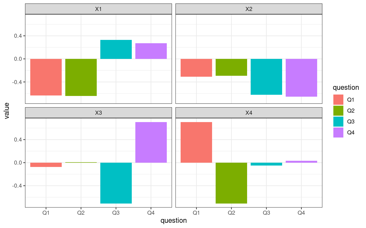

Example: Human abilities

Let’s look at another slightly more complex (real) data set: one on human abilities. We will use ability.cov–the covariance of these abilities, and convert it to a correlation matrix:

library(GPArotation)
data(ability.cov)
e2 <- eigen(cov2cor(ability.cov$cov))
plot(e2$values)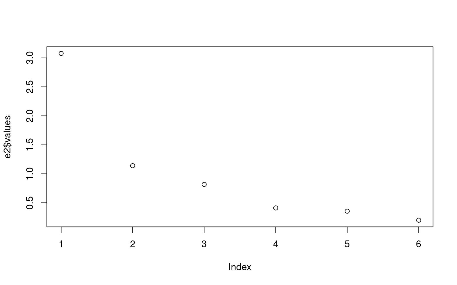

evec <- e2$vectors
rownames(evec) <- rownames(ability.cov$cov)
round(evec, 3)

          [,1]   [,2]   [,3]   [,4]   [,5]   [,6]
general -0.471  0.002  0.072  0.863  0.037 -0.164
picture -0.358  0.408  0.593 -0.268  0.531  0.002
blocks  -0.434  0.404  0.064 -0.201 -0.775  0.051
maze    -0.288  0.404 -0.794 -0.097  0.334  0.052
reading -0.440 -0.507 -0.015 -0.100  0.056  0.733
vocab   -0.430 -0.501 -0.090 -0.352  0.021 -0.657

dvec <- data.frame(evec)
dvec$test <- rownames(dvec)

Here, there is a large drop-off between 1 and 2 eigenvalues, but it really flattens out after 3 dimensions. We can show each vector as follows:

dvec %>%
    pivot_longer(X1:X6, names_to = "Component") %>%
    ggplot(aes(x = Component, y = value, group = test, fill = test), position = "dodge") +
    geom_col(position = "dodge", color = "grey25")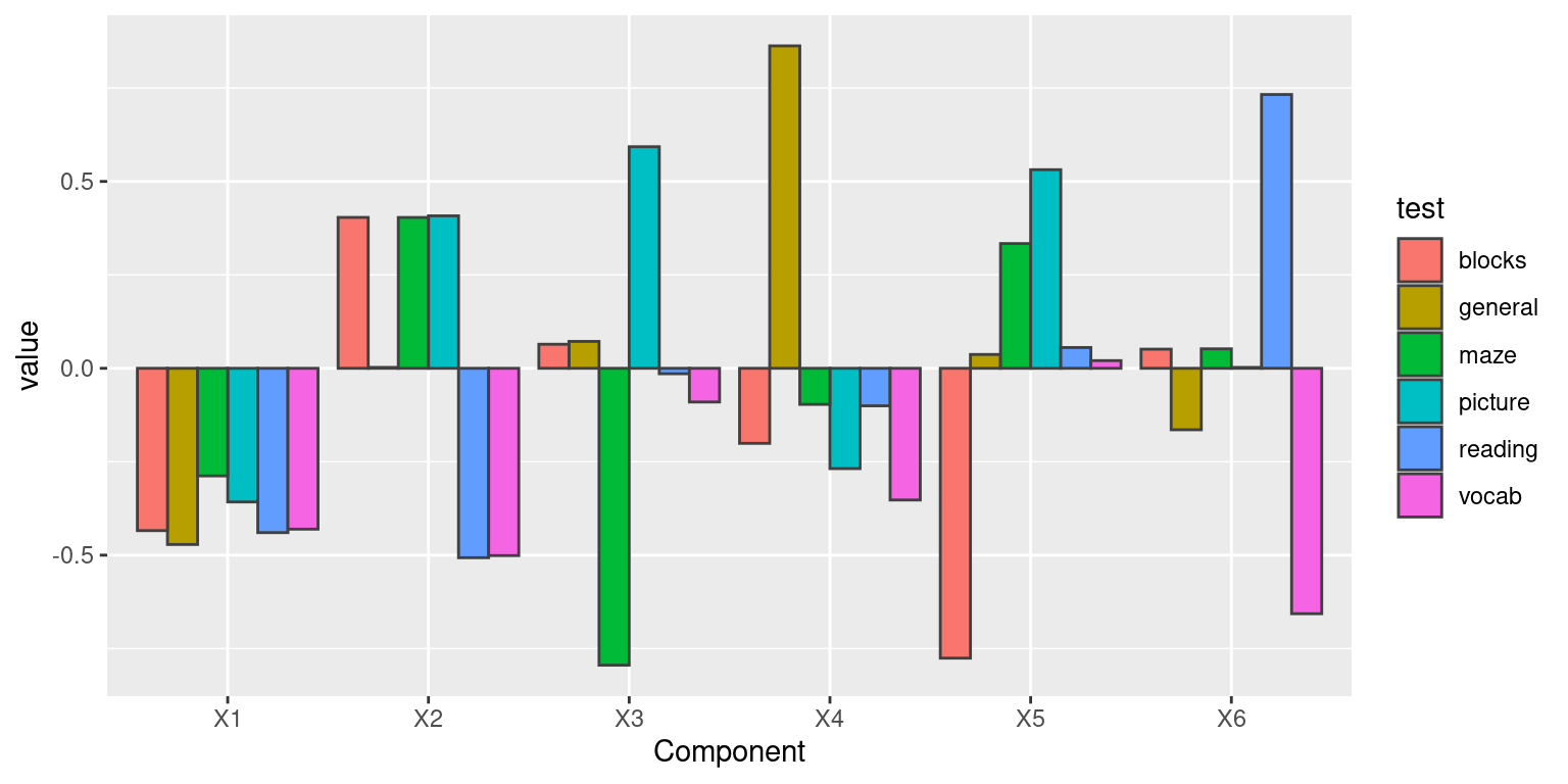

Looking at the eigenvectors, vector values that are different from 0 indicate a high positive or negative involvement of a particular question in a particular factor. Here, the first factor is generally equally involved in each question–maybe general intelligence. This makes sense if you look at the covariance, because there is a lot of positive correlation among the whole set. The negative value has no real meaning. The second factor is blocks, maze, picture vs reading/vocab; maybe visual versus lexical intelligence. This is one way of carving up the fact that there might be a general intelligence that impacts everyone, and a second factor that isn’t general but might be visual or vocabulary. This is a bit misleading though–if someone is good at both or bad at both, it gets explained as general intelligence; if they are good or bad at one or the other, it gets explained as a specific type of intelligence. After this, each remaining vector essentially picks out a pair of tests to contrast. Note that although the values can be large, the importance gets scaled by the eigenvalue, and so the amount of variance accounted for is really quite small.

Looking at this, a hierarchical structure appears, which might indicate a hierarchical clustering would be better. We will cover this approach in later work, but for the moment I’ll create a distance measure from the covariance converting to a correlation and subtracting from 1.0.

library(cluster)

cor <- ability.cov$cov/sqrt(diag(ability.cov$cov) %*% t(diag(ability.cov$cov)))
dist <- as.dist(1 - cor)
a <- agnes(dist)
plot(a, which = 2)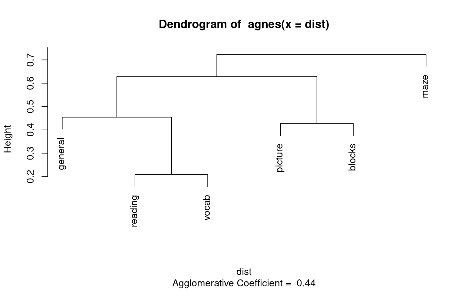

This sort of maps onto our intuition; maze here looks like a bit of an outlier.

Using the princomp and prcomp, and principal functions

The princomp and prcomp functions are included in R, and does the same thing as eigen(), with a few additional bells and whistles. Notice that the vectors are identical. Another option in the psych::principal function.

p <- princomp(covmat = cov2cor(ability.cov$cov))
plot(p)
summary(p)

Importance of components:
                          Comp.1    Comp.2    Comp.3     Comp.4     Comp.5
Standard deviation     1.7540877 1.0675615 0.9039839 0.64133665 0.59588119
Proportion of Variance 0.5128039 0.1899479 0.1361978 0.06855212 0.05917907
Cumulative Proportion  0.5128039 0.7027518 0.8389497 0.90750178 0.96668085
                           Comp.6
Standard deviation     0.44711845
Proportion of Variance 0.03331915
Cumulative Proportion  1.00000000

loadings(p)


Loadings:
        Comp.1 Comp.2 Comp.3 Comp.4 Comp.5 Comp.6
general  0.471                0.863         0.164
picture  0.358  0.408  0.593 -0.268  0.531       
blocks   0.434  0.404        -0.201 -0.775       
maze     0.288  0.404 -0.794         0.334       
reading  0.440 -0.507        -0.100        -0.733
vocab    0.430 -0.501        -0.352         0.657

               Comp.1 Comp.2 Comp.3 Comp.4 Comp.5 Comp.6
SS loadings     1.000  1.000  1.000  1.000  1.000  1.000
Proportion Var  0.167  0.167  0.167  0.167  0.167  0.167
Cumulative Var  0.167  0.333  0.500  0.667  0.833  1.000

screeplot(p)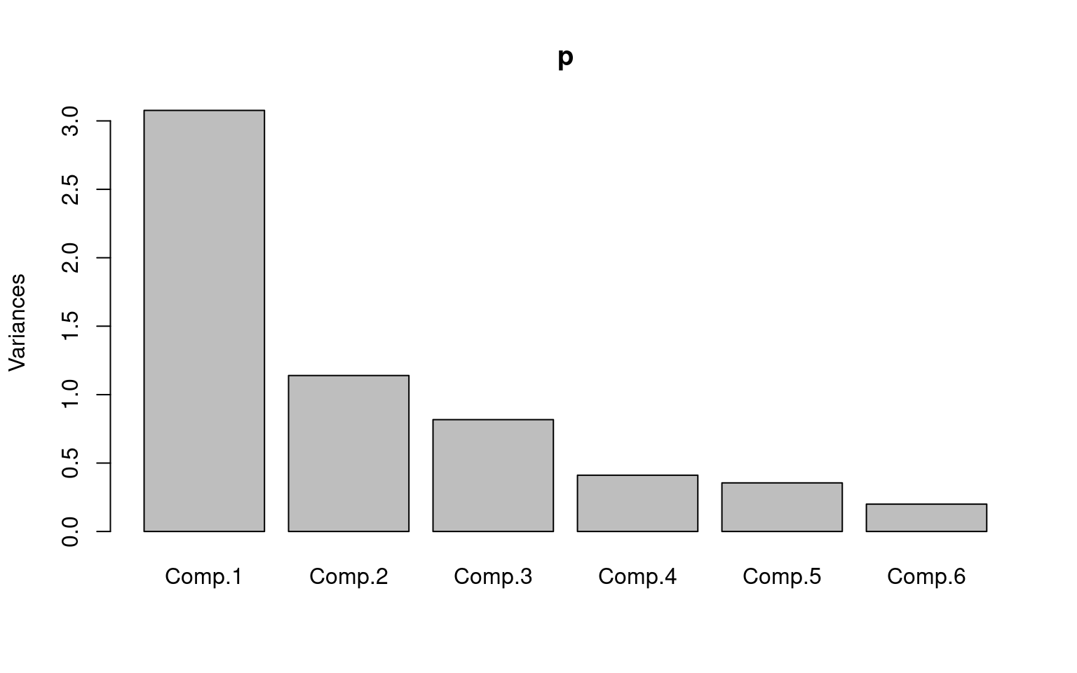

The advantage of princomp is that it lets you use the raw data, and will compute scores based on those base data. There is a related function called prcomp, which will do a similar analysis, but handles situations where you have fewer participants than questions.

The psych library (which we will use again a number of times) has the function principal, but frames it within the psych factor analysis functions, which provide much more detailed output. Here, you must specify the number of factors from the outset, and the solutions appear to change a bit when you do so. The solution doesn’t really change, but the vectors get rescaled.

p2 <- psych::principal(r = cov2cor(ability.cov$cov), nfactors = 4)
print(p2)

Principal Components Analysis
Call: psych::principal(r = cov2cor(ability.cov$cov), nfactors = 4)
Standardized loadings (pattern matrix) based upon correlation matrix
         RC2  RC4   RC3  RC1   h2     u2 com
general 0.35 0.31  0.18 0.86 0.99 0.0059 1.7
picture 0.10 0.93 -0.01 0.16 0.90 0.1003 1.1
blocks  0.21 0.71  0.42 0.22 0.79 0.2141 2.1
maze    0.09 0.12  0.96 0.12 0.96 0.0401 1.1
reading 0.89 0.13  0.05 0.27 0.89 0.1084 1.2
vocab   0.93 0.13  0.12 0.12 0.91 0.0863 1.1

                       RC2  RC4  RC3  RC1
SS loadings           1.85 1.52 1.15 0.92
Proportion Var        0.31 0.25 0.19 0.15
Cumulative Var        0.31 0.56 0.75 0.91
Proportion Explained  0.34 0.28 0.21 0.17
Cumulative Proportion 0.34 0.62 0.83 1.00

Mean item complexity =  1.4
Test of the hypothesis that 4 components are sufficient.

The root mean square of the residuals (RMSR) is  0.05 

Fit based upon off diagonal values = 0.98

Exercise: Big five data

Do a PCA of the big five data:

data <- read.csv("bigfive.csv")

dat.vals <- data[, -1]  ##remove subject code
qtype <- c("E", "A", "C", "N", "O", "E", "A", "C", "N", "O", "E", "A", "C", "N",
    "O", "E", "A", "C", "N", "O", "E", "A", "C", "N", "O", "E", "A", "C", "N", "O",
    "E", "A", "C", "N", "O", "E", "A", "C", "N", "O", "O", "A", "C", "O")
valence <- c(1, -1, 1, 1, 1, -1, 1, -1, -1, 1, 1, -1, 1, 1, 1, 1, 1, -1, 1, 1, -1,
    1, -1, -1, 1, 1, -1, 1, 1, 1, -1, 1, 1, -1, -1, 1, -1, 1, 1, 1, -1, 1, -1, 1)
add <- c(6, 0, 0)[valence + 2]


tmp <- dat.vals
tmp[is.na(tmp)] <- 3
reversed <- t(t(tmp) * valence + add)
## reverse code questions:

bytype <- reversed[, order(qtype)]
key <- sort(qtype)
colnames(bytype) <- paste(key, 1:44, sep = "")

Here is one way to visualize what PCA does. We can make an image plot of the correlation matrix of these questions. Because they are ordered, we see bands in the image:

pc <- princomp(bytype)
plot(pc)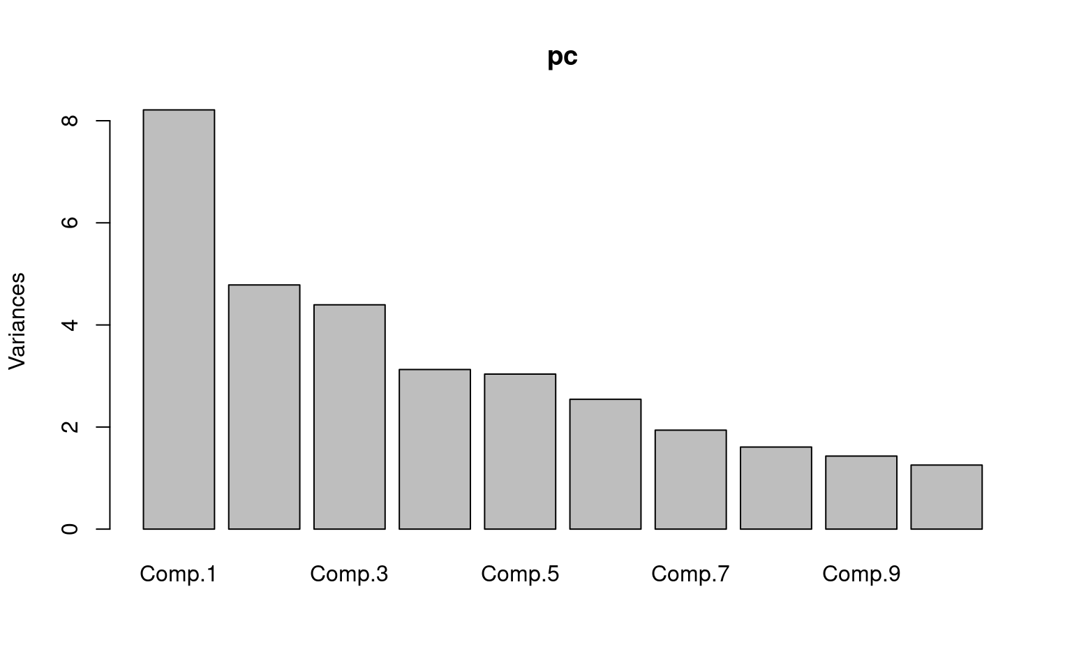

cbt <- cor(bytype)
image(cbt, col = grey(100:0/100))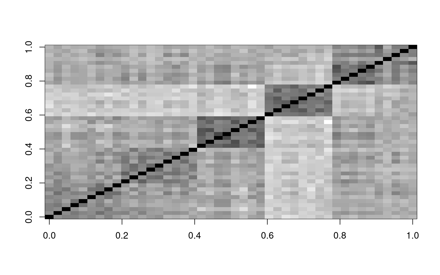

loadings(pc)


Loadings:
    Comp.1 Comp.2 Comp.3 Comp.4 Comp.5 Comp.6 Comp.7 Comp.8 Comp.9 Comp.10
A1   0.148  0.121         0.119  0.160  0.141  0.335         0.116  0.191 
    Comp.11 Comp.12 Comp.13 Comp.14 Comp.15 Comp.16 Comp.17 Comp.18 Comp.19
A1   0.141   0.132                   0.263                   0.469   0.263 
    Comp.20 Comp.21 Comp.22 Comp.23 Comp.24 Comp.25 Comp.26 Comp.27 Comp.28
A1   0.393                           0.283                   0.171         
    Comp.29 Comp.30 Comp.31 Comp.32 Comp.33 Comp.34 Comp.35 Comp.36 Comp.37
A1                           0.125                   0.133                 
    Comp.38 Comp.39 Comp.40 Comp.41 Comp.42 Comp.43 Comp.44
A1                                                         
 [ reached getOption("max.print") -- omitted 43 rows ]

               Comp.1 Comp.2 Comp.3 Comp.4 Comp.5 Comp.6 Comp.7 Comp.8 Comp.9
SS loadings     1.000  1.000  1.000  1.000  1.000  1.000  1.000  1.000  1.000
               Comp.10 Comp.11 Comp.12 Comp.13 Comp.14 Comp.15 Comp.16 Comp.17
SS loadings      1.000   1.000   1.000   1.000   1.000   1.000   1.000   1.000
               Comp.18 Comp.19 Comp.20 Comp.21 Comp.22 Comp.23 Comp.24 Comp.25
SS loadings      1.000   1.000   1.000   1.000   1.000   1.000   1.000   1.000
               Comp.26 Comp.27 Comp.28 Comp.29 Comp.30 Comp.31 Comp.32 Comp.33
SS loadings      1.000   1.000   1.000   1.000   1.000   1.000   1.000   1.000
               Comp.34 Comp.35 Comp.36 Comp.37 Comp.38 Comp.39 Comp.40 Comp.41
SS loadings      1.000   1.000   1.000   1.000   1.000   1.000   1.000   1.000
               Comp.42 Comp.43 Comp.44
SS loadings      1.000   1.000   1.000
 [ reached getOption("max.print") -- omitted 2 rows ]

Approximating the correlation matrix with a small number of factors.

In the image above, the darker colors indicate a higher correlation. There are bands/squares, indicating questions that go together. The eigen doesn’t give is this order–we pre-sorted the like questions to go together.

When we use eigen decomposition, we are breaking the correlation into independent elements. We can recompute the main correlational structure from each element by taking the cross product of each factor with itself. Then, by adding these together (in the proportion specified by the eigenvalues), we can re-represent the original correlation matrix. If we have 45 variables, we can then look at how much of the original structure we can reproduce from a small number of factors.

Suppose we had a vector that picked out the each personality factor, one at a time.

length <- length(key)
noise <- 0.1
f.a <- (key == "A") + runif(length(key)) * noise
f.c <- (key == "C") + runif(length(key)) * noise
f.e <- (key == "E") + runif(length(key)) * noise
f.n <- (key == "N") + runif(length(key)) * noise
f.o <- (key == "O") + runif(length(key)) * noise

If we compute expected correlation if everything within a group was the same, we can do that by using a matrix product

cor.a <- f.a %*% t(f.a)
cor.c <- f.c %*% t(f.c)
cor.e <- f.e %*% t(f.e)
cor.n <- f.n %*% t(f.n)
cor.o <- f.o %*% t(f.o)
image(cor.a, col = grey(100:0/100))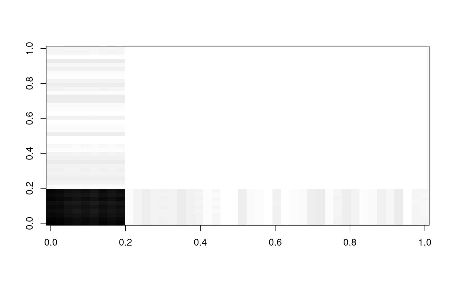

image(cor.c, col = grey(100:0/100))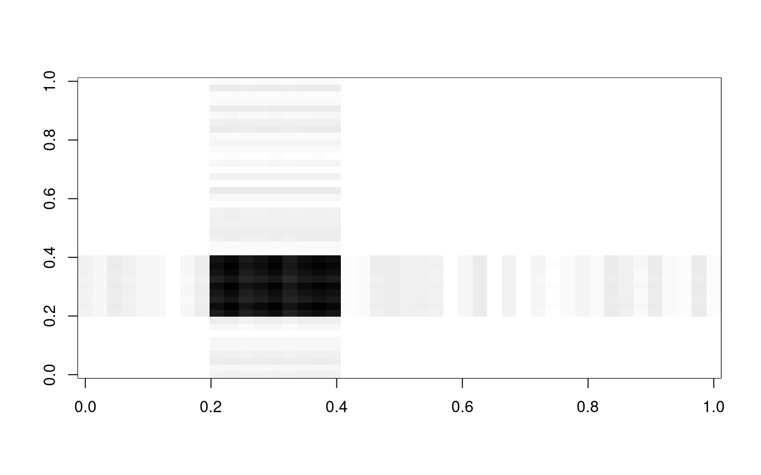

image(cor.e, col = grey(100:0/100))

image(cor.n, col = grey(100:0/100))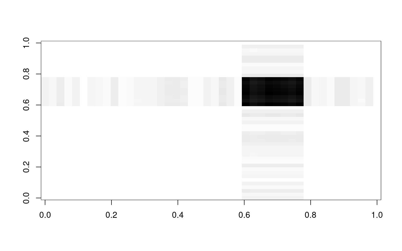

image(cor.o, col = grey(100:0/100))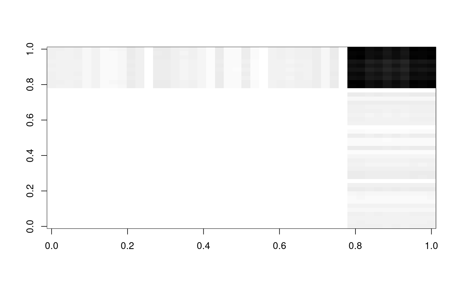

If we add each of these up, we approximate the original correlation matrix

par(mfrow = c(1, 2))
image(cor.a + cor.c + cor.e + cor.n + cor.o, col = grey(100:0/100))
image(cbt, col = grey(100:0/100))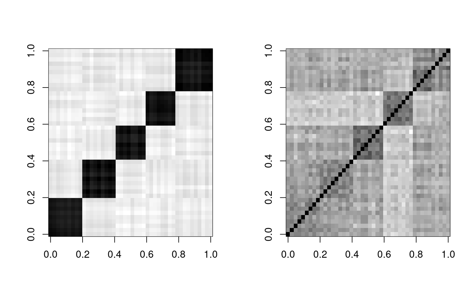

So, on the left is our faked factor with a little noise, which maps exactly onto our big-five theory. On the right is the truth. These resemble one another, although not perfectly. We can do this with the real data and real factors obtained via PCA. That is the basic idea of PCA, and factor analysis in general–to find factors like f.n, f.o, etc that will recombine to model the correlation matrix. PCA finds these factors for you, and the really amazing thing about PCA is that the top few factors will usually reconstruct the matrix fairly well, with the noise being captured by the less important eigenvectors.

e <- eigen(cbt)
par(mfrow = c(2, 3))
image(cbt, col = grey(100:0/100), main = "Complete correlation")
image((e$vectors[, 1] * t(e$values[1])) %*% t(e$vectors[, 1]), col = grey(100:0/100),
    main = "One eigenvector")
image((e$vectors[, 1:2] * (e$values[1:2])) %*% t(e$vectors[, 1:2]), col = grey(100:0/100),
    main = "Two eigenvectors")
image((e$vectors[, 1:3] * (e$values[1:3])) %*% t(e$vectors[, 1:3]), col = grey(100:0/100),
    main = "Three eigenvectors")
image((e$vectors[, 1:4] * (e$values[1:4])) %*% t(e$vectors[, 1:4]), col = grey(100:0/100),
    main = "Four eigenvectors")
image((e$vectors[, 1:5] * (e$values[1:5])) %*% t(e$vectors[, 1:5]), col = grey(100:0/100),
    main = "Five eigenvectors")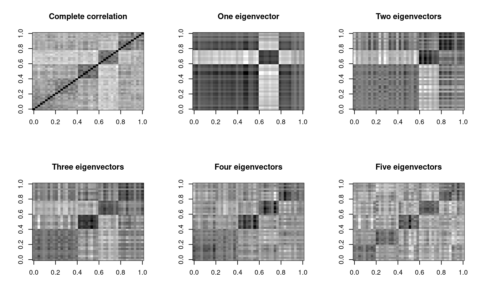

par(mfrow = c(1, 2))
image(cbt, col = grey(100:0/100), main = "Complete correlation")
image((e$vectors[, 1:10] * e$values[1:10]) %*% t(e$vectors[, 1:10]), col = grey(100:0/100),
    main = "Ten eigenvectors")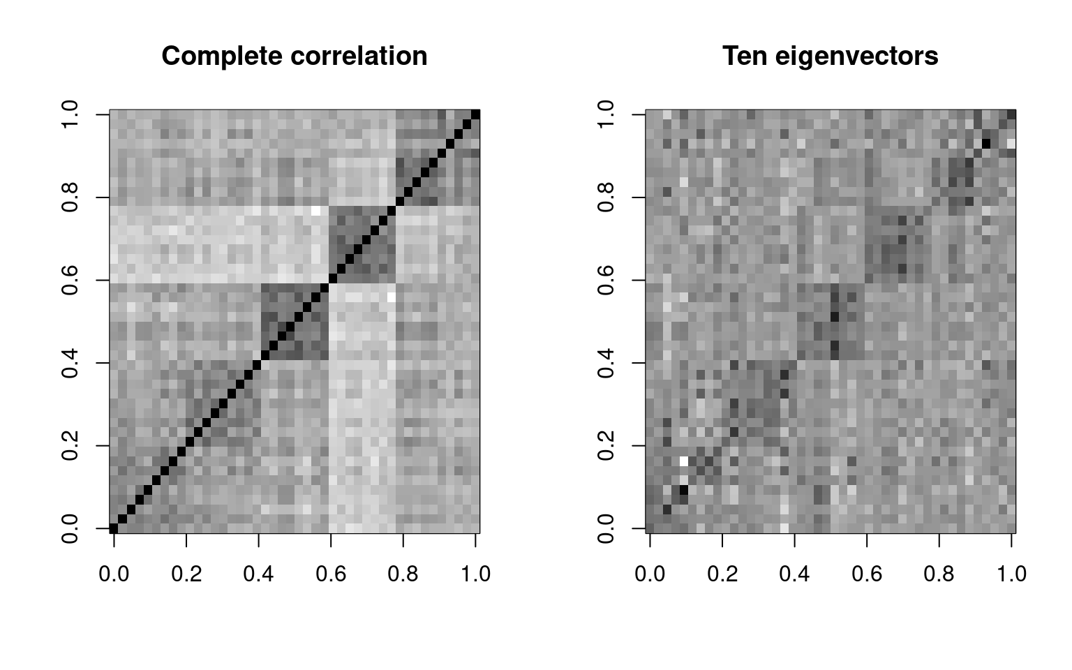

By the time we use five eigenvectors, the matrix gets to be fairly similar to the original. This is 5 out of 44 possible vectors, so we are compressing the data down by a factor of nearly 90%, finding just the important things, and throwing out everything else–treating it as noise. Also shown above is what we get if we go up to 10 factors–not much better than 5.

This might resemble image or audio compression if you are familiar with how these work. In fact, they are quite similar! Projecting to a subspace could alternately be referred to as compressing data.

Eigen decomposition versus SVD

To do the PCA, we essentially did two steps: first computing correlation or covariance, and then eigen decomposition of that covariance matrix. There is a alternative process that computes a similar decomposition using the raw feature data, called Singular Value Decomposition (SVD). Some PCA or Factor Analysis methods use SVD, and it can be used effectively for very large data sets, where it is intractable to compute a complete correlation matrix. Oftentimes, an SVD will be done and a researcher will report the results as a PCA.

Let’s compare the eigen decomposition to the SVD on the raw data; using 5-features. The original data was ’‘’bytype’’‘, and the correlation matrix was’‘’cbt’’’. Let’s bypass the cbt matrix:

factors1 <- eigen(cov(bytype))

## a 15-factor solution using SVD
factors2 <- svd(bytype, nu = 15)
summary(factors1)

        Length Class  Mode   
values    44   -none- numeric
vectors 1936   -none- numeric

summary(factors2)

  Length Class  Mode   
d    44  -none- numeric
u 15255  -none- numeric
v  1936  -none- numeric

The eigen decomposes the square matrix into a vector 44 long and a square matrix. The svd decomposes into a vector and two rectangular matrices.

Here is the ‘scree’ plot for each–eigen values (variance) and the svd d matrix. Notice that the first factor of the SVD is much larger; this is in part because we have already normalized everything in PCA by using correlation. So the first dimension is essentially an ‘intercept’ term, which tries to get the overall level right. Removing this, the two screeplots look fairly similar.

par(mfrow = c(1, 3))
plot(factors1$values, main = "Eigen scree plot")
plot(factors2$d, main = "SVD scree plot")
plot(factors2$d[-1], main = "SVD scree plot removing first dimension")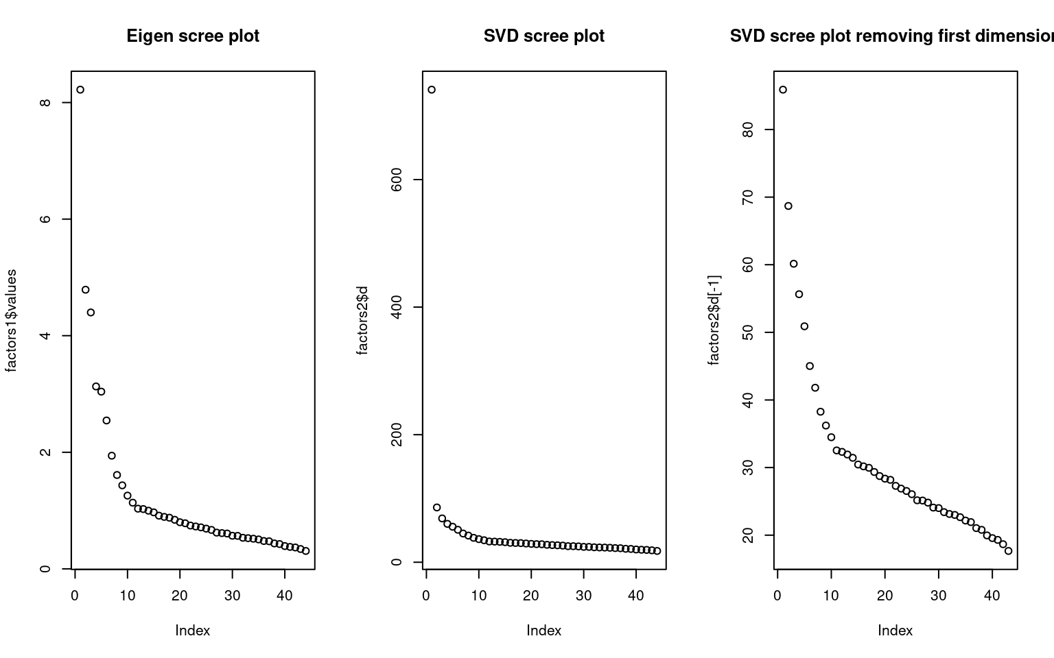

The first dimension of SVD is not very interesting here–just an intercept and because all terms were relatively similar, they do not differ by question:

barplot(factors2$v[, 1])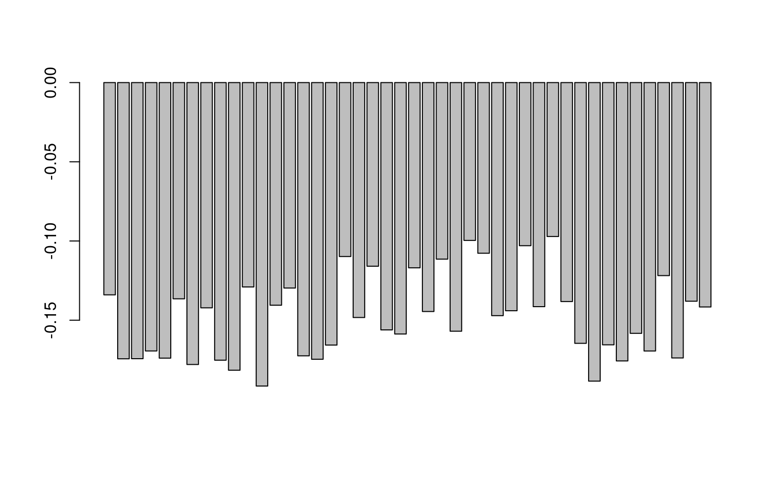

Following this, the remaining terms of SVD map onto the terms of eigen decomposition fairly well.

par(mfcol = c(4, 2))
barplot(factors1$vectors[, 1], main = "Eigen D1")
barplot(factors1$vectors[, 2], main = "Eigen D2")
barplot(factors1$vectors[, 3], main = "Eigen D3")
barplot(factors1$vectors[, 4], main = "Eigen D4")


barplot(factors2$v[, 2], main = "SVD D2")
barplot(factors2$v[, 3], main = "SVD D3")
barplot(factors2$v[, 4], main = "SVD D4")
barplot(factors2$v[, 5], main = "SVD D5")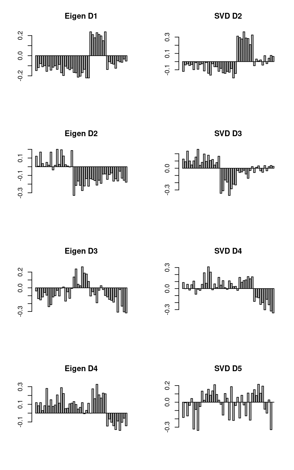

The results are not identical—computing the correlation of the data does normalization that removes some information that SVD uses, but the results are similar up to the first few dimensions.

We can calculate the correlation between the first ten factors of each.

cc <- cor(factors1$vectors, factors2$v)
round(((abs(cc) > 0.3) * cc)[1:10, 1:10], 3)

        [,1]   [,2]   [,3]  [,4]  [,5]   [,6]  [,7]   [,8]   [,9] [,10]
 [1,]  0.339  0.985  0.000 0.000 0.000  0.000  0.00  0.000  0.000 0.000
 [2,]  0.000 -0.315  0.872 0.334 0.000  0.000  0.00  0.000  0.000 0.000
 [3,]  0.443 -0.343 -0.690 0.590 0.000  0.000  0.00  0.000  0.000 0.000
 [4,]  0.339  0.000  0.000 0.868 0.000  0.000  0.00  0.000  0.000 0.000
 [5,] -0.405  0.000  0.000 0.000 0.975  0.000  0.00  0.000  0.000 0.000
 [6,]  0.513  0.000  0.000 0.000 0.000 -0.998  0.00  0.000  0.000 0.000
 [7,]  0.000  0.000  0.000 0.000 0.000  0.000 -0.95  0.000  0.000 0.000
 [ reached getOption("max.print") -- omitted 3 rows ]

Notice that when we correlate the two factor solutions and zero-out any below .3, there are a number of high correspondences: E1 versus S2; E2 vs S4, E3 vs -S3, etc. However, the correspondence is not exact, for a number of reasons. First, SVD solution will solve just the top n dimensions; which has the effect of ‘compressing’ into fewer dimension. Also, eigen decomposition throws out some data by using the correlation (and even the covariance) matrix.

By doing appropriate scaling, we can get much more similar (and essentially identical) values from the two methods.

Choosing between SVD and Eigen decomposition

In one sense, you never have to choose between these methods; eigen decomposition requires a square matrix, and SVD a rectangular matrix. If you have a square matrix (a distance or correlation matrix), then you use eigen decomposition; otherwise you might try SVD.

But if you have the rectangular matrix (data x features), you might choose to create the correlation matrix and then do eigen decomposition on that. This is a fairly typical approach, and it has the advantage that some factor analytic approaches will require this correlation/covariance structure as input, and permit others to easily understand what you are doing.

However, there are times when computing the complete correlation matrix is not feasible, and you would prefer to go directly from an itemxfeature matrix to a small set of implied features. One of the greatest sucesses of this approach is with a method called ‘Latent Semantic Analysis’. LSA does SVD on large termxdocument data matrices. For example2, imagine a text corpus with 1 million documents (rows) and 200,000 words or terms (columns). Computing the correlation of words by documents may be impossible–it is a matrix with 40 billion entries. And computing eigen decomposition on a 200,000 x 200,000 matrix may never finish. But reasonable implementation of SVD (ones available to academics in the 1980s and 1990s) could solve the SVD with 100-300 dimensions. LSA turns out to create a nice semantic space–words that tend to appear together in documents tend to have similar meaning, and it turns the co-occurrences into a feature space.

Summary

Within R, there are a number of related function that do PCA, and a number of decisions about how to do it.

Using eigen on either covariance or correlation matrix
using svd on raw data (possibly normalizing/scaling variables)
princomp, which uses eigen, with either covariance or correlation matrix
prcomp, which uses svd, with or without scaling variables
principal within the psych:: package does eigen decomposition and provides more readable output and goodness of fit statistics, with loadings rescaled by eigenvalues. This also permits using alternate rotations, which we will discuss in factor analysis sections.
factoextra functions (mostly useful for special-purpose graphing using ggplot2 and special analytics)
Routines in other libraries such as ade4, factomineR, and epPCA in ExPosition, which focuses on SVD.

In general, the different methods can probably all be made to give identical results with the right scaling, centering, and other assumptions. However, choosing between them depends on several factors:

Ease and value of interpretation, output, and statistics
Computational feasibility of computing eigen decomposition and correlation/covariance matrix on large data sets
If there are too few observations with respect to the number of questions, the correlation matrix across questions will be rank-deficient:it will necessarily contain fewer principal components than observations. In these cases, the prcomp svd will be able to produce a solution (although that solution might not be worth much because of the low number of observations).

Finally, principal components analysis useful for data processing, feature reduction, and the like; but for a more statistical analysis, scientists usually prefer a more complex set of related routines known colloquially as exploratory factor analysis.

Additional Example: Network flows

Suppose you had a network with different nodes and transition probabilities between nodes. For example, you might have three economic classes: poverty, middle-class, and wealthy. Any person from one generation has a certain probability of ending up in each of the other classes, maybe with a structure like this:

transition <- rbind(c(0.5, 0.5, 0), c(0.25, 0.5, 0.25), c(0, 0.5, 0.5))

For any generation of people, there is a distribution of class membership, and we can derive the subsequent distribution by cross-multiplying

dsn <- runif(3)

dsn <- dsn/sum(dsn)
overtime <- matrix(0, nrow = 100, ncol = 3)
overtime[1, ] <- dsn
for (i in 2:100) {
    dsn <- dsn %*% transition
    # dsn <- dsn/sum(dsn)
    overtime[i, ] <- dsn
}



matplot(overtime, ylim = c(0, 1), type = "o")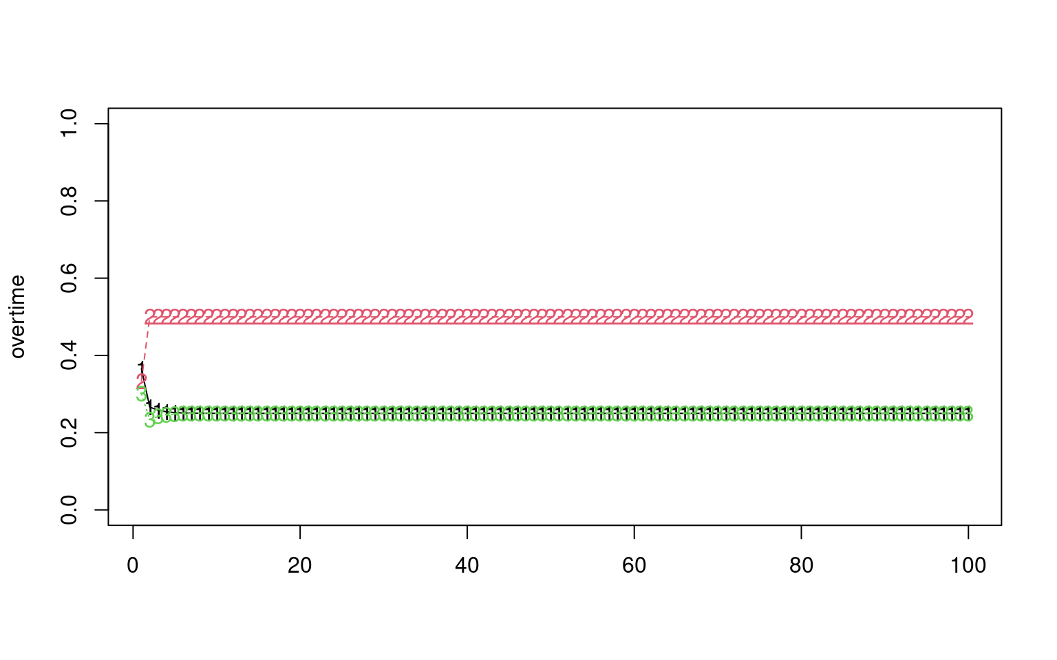

e <- eigen(t(transition))


print(e)

eigen() decomposition
$values
[1]  1.000000e+00  5.000000e-01 -7.019029e-17

$vectors
          [,1]          [,2]       [,3]
[1,] 0.4082483 -7.071068e-01  0.4082483
[2,] 0.8164966  8.112147e-16 -0.8164966
[3,] 0.4082483  7.071068e-01  0.4082483

print(dsn)

     [,1] [,2] [,3]
[1,] 0.25  0.5 0.25

Notice that the eigenvectors have one with all positive values, and it is (.4,.8,.4). If we normalize this, we get (.25, .5, .25), which is the stationary distribution of this stochastic matrix. Sometimes, there are multiple stable distributions depending on the starting conditions, and these would each map onto a distinct eigenvector. in this case, the second eigenvector is essentially -1,0,1; this vector cannot happen for a transition matrix (you can’t have negative probability), so in this case there are no other stable distributions.

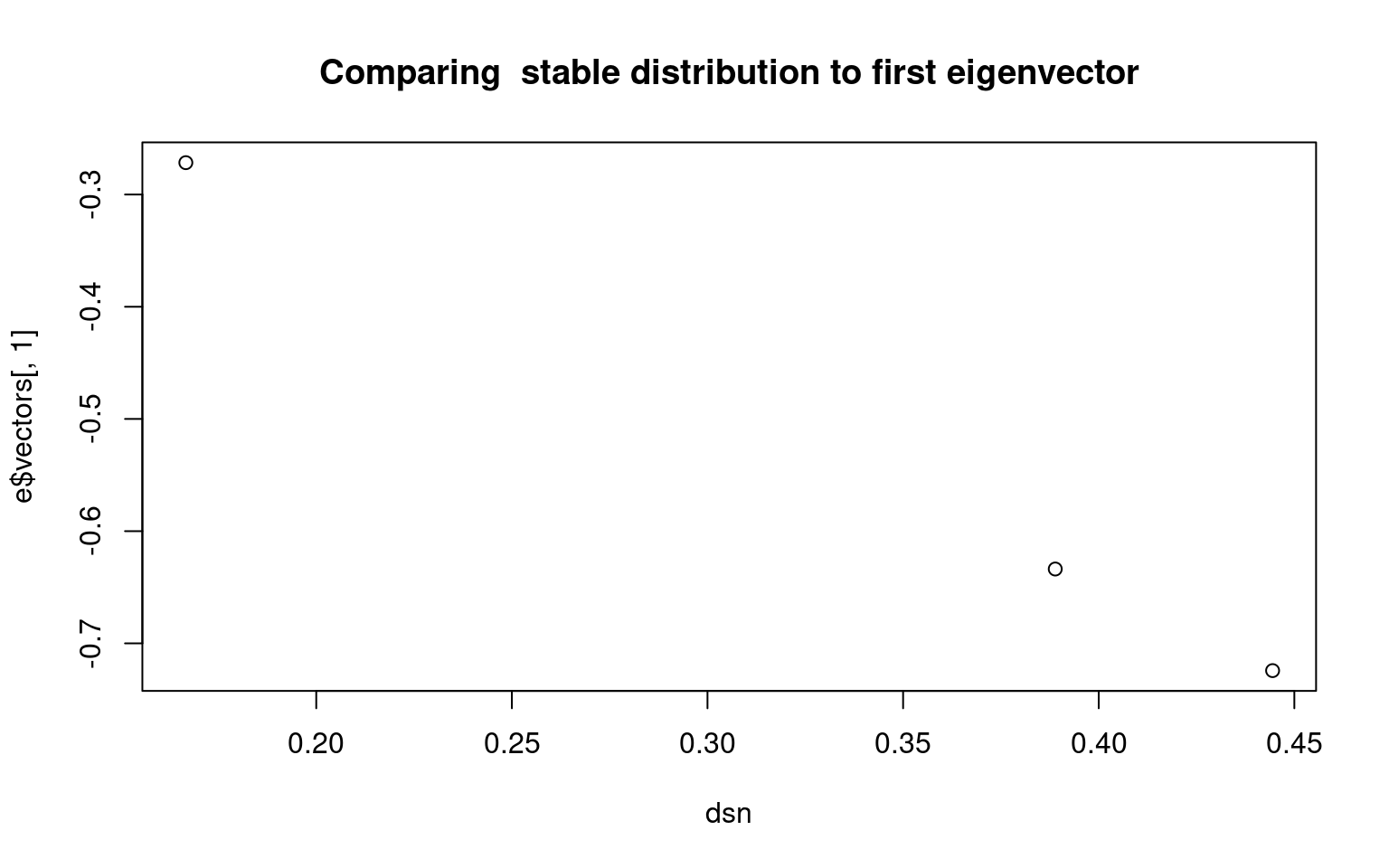
Here is another case where there is complete ability to transition between groups. Now, the first eigenvector is all negative, which also predicts the stationary distribution, at least ordinally.

transition <- rbind(c(0.5, 0.4, 0.1), c(0.4, 0.5, 0.1), c(0.1, 0.4, 0.5))
e <- eigen(t(transition))
print("Eigen decomposition:")

[1] "Eigen decomposition:"

print(e)

eigen() decomposition
$values
[1] 1.0 0.4 0.1

$vectors
           [,1]          [,2]          [,3]
[1,] -0.6337502 -7.071068e-01 -7.071068e-01
[2,] -0.7242860  2.266233e-16  7.071068e-01
[3,] -0.2716072  7.071068e-01  3.462330e-17

e$vectors[, 1]/sum(e$vectors[, 1])

[1] 0.3888889 0.4444444 0.1666667

dsn <- runif(3)

dsn <- dsn/sum(dsn)
overtime <- matrix(0, nrow = 100, ncol = 3)
overtime[1, ] <- dsn
for (i in 2:100) {
    dsn <- dsn %*% transition
    # dsn <- dsn/sum(dsn)
    overtime[i, ] <- dsn
}


print("----------------------")

[1] "----------------------"

matplot(overtime, ylim = c(0, 1))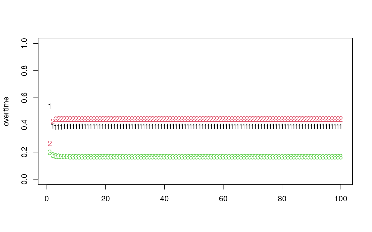

print("Stationary distribution:")

[1] "Stationary distribution:"

print(dsn)

          [,1]      [,2]      [,3]
[1,] 0.3888889 0.4444444 0.1666667

plot(dsn, e$vectors[, 1], main = "Comparing  stable distribution to first eigenvector")

PCA, eigen decomposition and SVD