Psychometrics: Validity and Reliability
Libraries used: psych, icc, irr, multilevel
Measures of Reliability and Validity
Reliability and validity go hand-in-hand when we are thinking about measuring a psychological concept. ‘’Reliability’’ refers to the extent to which your measure is reproducible, and likely to give you the same answer if you applied it twice (assuming you were able to apply it twice). ‘’Validity’’ refers to the extent to which the measure suits the purpose you are using it for. Many forms of both reliability and validity have been described, and although validity is typically a more conceptual property, both properties are established by looking at the psychometric properties of a measure.
We will look at several ways of assessing the psychometric properties of a test. As a first example, we will look at repeated measurement of the “trail-making” test.
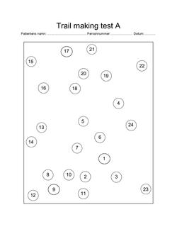
The trailmaking test. Patients play connect-the-dots, either with a series of numbers (Form A) or a mixed series of numbers and letters (Form B).
Test-retest, inter-rater, and inter-test reliability
If you want to know whether a test will give the same results if you measure it more than once, the simplest way to do this is to measure it twice and look at the correlation between the measures. This is known as test-retest reliability. Often, people will use standard correlation coefficients.
This can come in handy in several types of situations, including:
- When each person has taken the same test twice (maybe with delay)
- When you have developed different forms of a test and want to assess whether they measure the same thing.
- When you have two raters coding behavior and want to establish inter-rater reliability
- When you want to establish criterion validity of one measure against a second normed measure
- When you want to determine whether what you are measuring in the first five minutes of a test is the same as what an entire 30-minute test measures.
- Comparing one measure of a construct to another measure of a construct (e.g., executive function; spatial reasoning, etc.).
- Compare a computerized test to a paper-and-pencil test
Using the correlation coefficient
To establish reliability, the simplest approach is to compute the correlation between your two measures. If your variables are significantly non-normal (e.g., highly-skewed), you might use a spearman (rank-order) correlation instead of a continuous Pearson correlation. If your two measures are likely to be on different scales (e.g., if you are comparing one existing measure of vision to a new measure of vision), this is also appropriate, but recognize that a high correlation does not mean the two measures have the same values. For example, if you gave a physics test twice, you might get a high correlation across test-takers, but the second test might have higher scores.
Consider the following data set using several related measures of the trail-making test (TMT). In this study, participants completed 9 TMT measures. The TMT involves doing a connect-the-dots test, and compares one (Form A) that is just letters A-B-C-D, and a second (Form B) that rotates between letters and number (A-1-B-2-…). First, they completed the standard Reitan paper-and-pencil test, initially Form A and then Form B. However, along with having a different layout, these forms are also of different lengths and complexities, which is a problem for the test—but one most people ignore (even though it is one of the most widely used cognitive tests in existence). To help develop a better alternative, we then had participants solve four versions of the test via computer–two each for both layouts in both letter conditions. Finally, several additional new randomly-generated tests were completed to provide independent pure and switch scores. We are interested in whether the different versions in either a switch or a non-switch condition have high test-retest validity–do they measure similar things?
library(ggplot2)
library(GGally)  ##GGally is a front-end to ggplot that will make the pairs plot equivalent
library(reshape2)
tmt <- read.csv("trailmaking.csv")
# pairs(tmt[,-1])
ggpairs(tmt[, -1], progress = FALSE)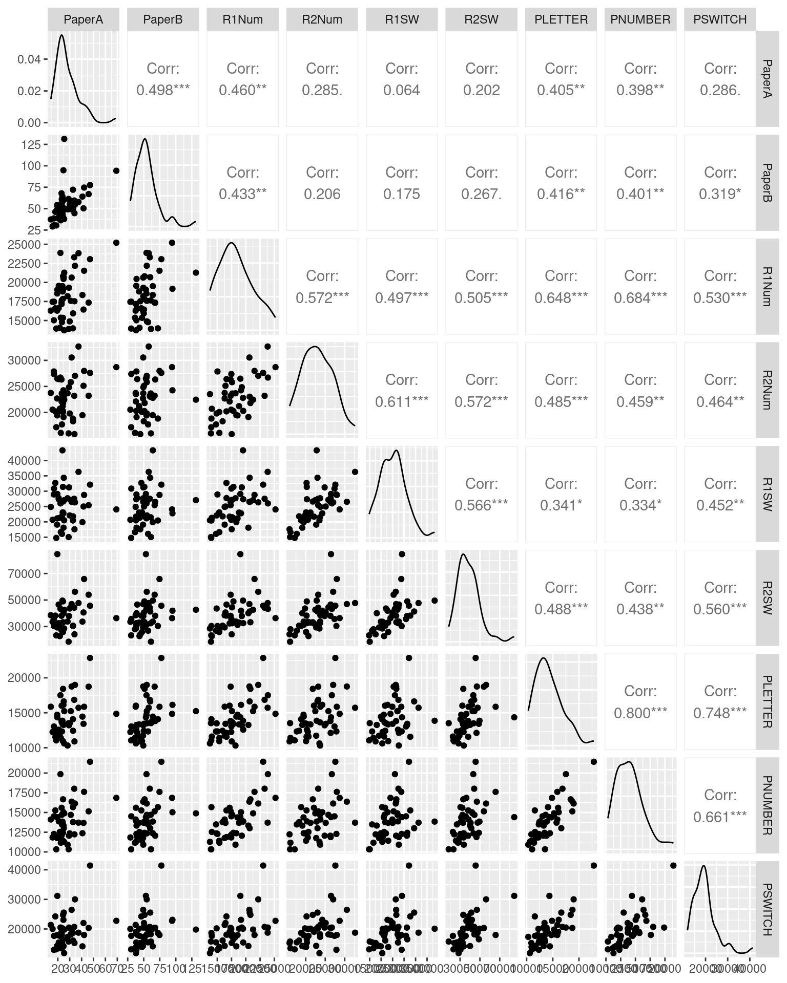
# library(knitr)
knitr::kable(round(cor(tmt[, -1]), 2), caption = "Pearson Inter-correlations between different trail-making tests")| PaperA | PaperB | R1Num | R2Num | R1SW | R2SW | PLETTER | PNUMBER | PSWITCH | |
|---|---|---|---|---|---|---|---|---|---|
| PaperA | 1.00 | 0.50 | 0.46 | 0.29 | 0.06 | 0.20 | 0.40 | 0.40 | 0.29 |
| PaperB | 0.50 | 1.00 | 0.43 | 0.21 | 0.18 | 0.27 | 0.42 | 0.40 | 0.32 |
| R1Num | 0.46 | 0.43 | 1.00 | 0.57 | 0.50 | 0.50 | 0.65 | 0.68 | 0.53 |
| R2Num | 0.29 | 0.21 | 0.57 | 1.00 | 0.61 | 0.57 | 0.48 | 0.46 | 0.46 |
| R1SW | 0.06 | 0.18 | 0.50 | 0.61 | 1.00 | 0.57 | 0.34 | 0.33 | 0.45 |
| R2SW | 0.20 | 0.27 | 0.50 | 0.57 | 0.57 | 1.00 | 0.49 | 0.44 | 0.56 |
| PLETTER | 0.40 | 0.42 | 0.65 | 0.48 | 0.34 | 0.49 | 1.00 | 0.80 | 0.75 |
| PNUMBER | 0.40 | 0.40 | 0.68 | 0.46 | 0.33 | 0.44 | 0.80 | 1.00 | 0.66 |
| PSWITCH | 0.29 | 0.32 | 0.53 | 0.46 | 0.45 | 0.56 | 0.75 | 0.66 | 1.00 |
The Spearman rank-order correlation might be better because these are times, which are likely to be skewed positive:
knitr::kable(round(cor(tmt[, -1], method = "spearman"), 2), caption = "Spearman rank-order correlations")| PaperA | PaperB | R1Num | R2Num | R1SW | R2SW | PLETTER | PNUMBER | PSWITCH | |
|---|---|---|---|---|---|---|---|---|---|
| PaperA | 1.00 | 0.61 | 0.36 | 0.16 | 0.07 | 0.32 | 0.40 | 0.30 | 0.22 |
| PaperB | 0.61 | 1.00 | 0.41 | 0.21 | 0.20 | 0.41 | 0.59 | 0.45 | 0.41 |
| R1Num | 0.36 | 0.41 | 1.00 | 0.51 | 0.53 | 0.63 | 0.64 | 0.61 | 0.54 |
| R2Num | 0.16 | 0.21 | 0.51 | 1.00 | 0.64 | 0.62 | 0.46 | 0.42 | 0.50 |
| R1SW | 0.07 | 0.20 | 0.53 | 0.64 | 1.00 | 0.69 | 0.33 | 0.35 | 0.49 |
| R2SW | 0.32 | 0.41 | 0.63 | 0.62 | 0.69 | 1.00 | 0.63 | 0.51 | 0.64 |
| PLETTER | 0.40 | 0.59 | 0.64 | 0.46 | 0.33 | 0.63 | 1.00 | 0.77 | 0.70 |
| PNUMBER | 0.30 | 0.45 | 0.61 | 0.42 | 0.35 | 0.51 | 0.77 | 1.00 | 0.64 |
| PSWITCH | 0.22 | 0.41 | 0.54 | 0.50 | 0.49 | 0.64 | 0.70 | 0.64 | 1.00 |
Here, the rank-order Spearman correlation coefficient is a little higher (on average, about .027), but a lot higher for the Paper A versus B (.61 versus .49). We can use these correlations to examine the extent to which we have high positive correlations between forms.
ggplot(tmt, aes(x = PaperA, y = PaperB)) + geom_point()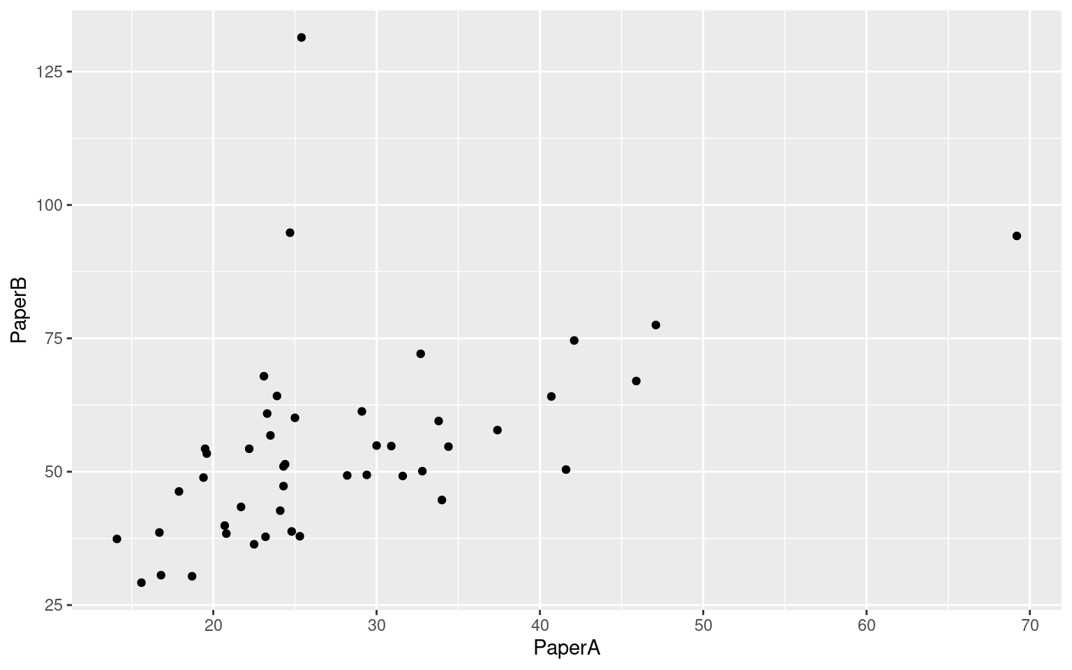
Results show:
- Correlation of .61 between form A and B paper tests
- Low correlation between paper and computer versions of the same problem. Here, form A paper is identical to R1Num (\(R=.36\)), and Form B paper is identical to R2SW (\(R=.414\)).
- The only correlations that start getting interesting are between computerized tests.
- Two forms of the simple PEBL Test were letter and number. Their correlation was +.8, indicating fairly good alternative-form reliability. The correlated moderately strongly with other computerized measures, and less well with the paper-and-pencil tests.
- Tests requiring a switch do not stand out as especially related to one another.
Intra-class Correlation Coefficients
When measures are on the same scale, you should use intraclass correlation coefficient (ICC), which was described by Shrout and Fleiss (1979). They identified 6 different ICC estimates for different designs, including having more than 2 raters. These are available in several different libraries:
* The psych library includes ICC1, ICC2, and ICC3. * The ICC library includes ICCbareF, ICCbare (which is more flexible), and ICCest (which provides confidence regions) for a one-way model (ICC1) * The multilevel library which includes ICC1 and ICC2. * The irr library includes icc for oneway and twoway models, reporting significance tests.
The different libraries generally calculate the same values, but have different ways of specifying the models, and their help files are sometimes inconsistent with one another. This is quite a rats nest to navigate. These different implementations are likely to handle missing data differently and require different input values, and it is not clear which apply to which ICC models—so be careful about reading the documentation. Let’s try to walk through the different kinds of ICC estimates.
To understand how ICC works, think about fitting an ANOVA model to your set of ratings, and computing an \(R^2\) of the overall model. A number of effect sizes (\(\eta^2\), partial \(\eta^2\), etc.) can be calculated by finding the proportion of variance accounted for by any argument and dividing by a sum of other variances. ICC is a similar calculation, and the different kinds of ICC use different pooled variance sums.
To start with, let’s refer to the people producing the values as raters, and the things being rated as targets (some refer to these as subjects). In our tmt task, we could calculate ICC by considering all the participants as raters and the tasks as targets, or each task as a different ‘rater’ and each participant as a target. These will tell us different things.
For an ICC-1, or one-way model, you essentially do a considers the targets as randomly sampled. A two-way model (ICC-2) considers the raters random–you might have a different set of raters for each judgement. It is impacted by differences in means (biases) between raters, so if one rater is strict and the other is lax, ICC will be low.
To examine this, we will look at TMT scales PNUMBER and PLETTER, which have similar completion times. We will consider each scale the result of a ‘rater’. Note that the correlation between these is .8 with a \(R^2\) of .64, and the best-fit line has a slope of .89–close to 1.0. But there is little consistency across people–some people have high scores and others have low scores. If we specify the model incorrectly, we are likely to get a very low number. The problem with ICC is that it is easy to specify the model incorrectly. We will start by creating two data frames and
library(tidyverse)
tmp <- tmt %>%
    dplyr::select(Subject, PLETTER, PNUMBER)
tmplong <- tmp %>%
    pivot_longer(cols = 2:3)

cor(tmp[, 2:3])^2
PLETTER PNUMBER
PLETTER 1.0000000 0.6404437
PNUMBER 0.6404437 1.0000000lm <- lm(tmt$PLETTER ~ tmt$PNUMBER)
summary(lm)
Call:
lm(formula = tmt$PLETTER ~ tmt$PNUMBER)

Residuals:
    Min      1Q  Median      3Q     Max
-3778.9 -1208.1  -232.4   926.0  3492.1

Coefficients:
             Estimate Std. Error t value Pr(>|t|)
(Intercept) 1798.2614  1421.0171   1.265    0.212
tmt$PNUMBER    0.8874     0.1002   8.853 2.49e-11 ***
---
Signif. codes:  0 '***' 0.001 '**' 0.01 '*' 0.05 '.' 0.1 ' ' 1

Residual standard error: 1599 on 44 degrees of freedom
Multiple R-squared:  0.6404,    Adjusted R-squared:  0.6323
F-statistic: 78.37 on 1 and 44 DF,  p-value: 2.49e-11
First, we can calculate using the ICC library which is the simplest–it only will calculate the ICC1, which is not always what we want. It requires a ‘long’ data frame where you give it the rating value and a grouping variable specifying the fixed factor of target. Note that we have no reference to which rater (test) was which–we only know that each participant gave two ratings.
library(ICC)
## The tests are the raters
ICC::ICCest(x = Subject, y = value, data = tmplong)
$ICC
[1] 0.7964547
$LowerCI
[1] 0.6612699
$UpperCI
[1] 0.8817495
$N
[1] 46
$k
[1] 2
$varw
[1] 1282400
$vara
[1] 5017917## the participants are the 'raters'--normally the wrong estimate:
ICC::ICCbare(x = name, y = value, data = tmplong)[1] -0.0181023Here, we get an ICC of .79, but if we do the wrong ICC we get a value of -.018. The ‘wrong’ ICC is not exactly wrong, it is just saying that in terms of absolute agreement, the 46 independent ratings were not at all consistent–something we already knew, and not really relevant to comparing the two scales. Notice that we give the predictor we don’t care about, and ignore the one we care about for ICC1.
irr Library
The irr library is straightforward and wants a matrix with columns the raters and rows the targets. Because it specifies a matrix, it can calculate several modelsWe specify ‘oneway’ as the model to use.
library(irr)
## irr ICC1: this takes a matrix, rows is targets and columns is raters
irr::icc(tmp[, 2:3], model = "oneway", type = "consistency")
Single Score Intraclass Correlation
Model: oneway
Type : consistency
Subjects = 46
Raters = 2
ICC(1) = 0.796
F-Test, H0: r0 = 0 ; H1: r0 > 0
F(45,46) = 8.83 , p = 7.19e-12
95%-Confidence Interval for ICC Population Values:
0.661 < ICC < 0.882## ICC2:
irr::icc(tmp[, 2:3], model = "twoway", type = "consistency", unit = "single") Single Score Intraclass Correlation
Model: twoway
Type : consistency
Subjects = 46
Raters = 2
ICC(C,1) = 0.796
F-Test, H0: r0 = 0 ; H1: r0 > 0
F(45,45) = 8.81 , p = 1.13e-11
95%-Confidence Interval for ICC Population Values:
0.659 < ICC < 0.882## Average score
irr::icc(tmp[, 2:3], model = "twoway", type = "consistency", unit = "average") Average Score Intraclass Correlation
Model: twoway
Type : consistency
Subjects = 46
Raters = 2
ICC(C,2) = 0.886
F-Test, H0: r0 = 0 ; H1: r0 > 0
F(45,45) = 8.81 , p = 1.13e-11
95%-Confidence Interval for ICC Population Values:
0.795 < ICC < 0.937multilevel library
The multilevel library requires you to make an aov model first, then it calculates either ICC1 or ICC2 values.
library(multilevel)

## multilevel ICC1
model <- aov(value ~ Subject, data = tmplong)
multilevel::ICC1(model)
[1] -0.02194134multilevel::ICC2(model)[1] -79.85053The psych library
The psych library calculates them all for you, if you provide the data as a matrix. This appears the easiest to use and most comprehensive version:
library(psych)

## psych ICC (reports all ICC flavors)
psych::ICC(tmp[, 2:3])
Call: psych::ICC(x = tmp[, 2:3])
Intraclass correlation coefficients
type ICC F df1 df2 p lower bound upper bound
Single_raters_absolute ICC1 0.80 8.8 45 46 7.2e-12 0.66 0.88
Single_random_raters ICC2 0.80 8.8 45 45 1.1e-11 0.66 0.88
Single_fixed_raters ICC3 0.80 8.8 45 45 1.1e-11 0.66 0.88
Average_raters_absolute ICC1k 0.89 8.8 45 46 7.2e-12 0.80 0.94
Average_random_raters ICC2k 0.89 8.8 45 45 1.1e-11 0.80 0.94
Average_fixed_raters ICC3k 0.89 8.8 45 45 1.1e-11 0.80 0.94
Number of subjects = 46 Number of Judges = 2
See the help file for a discussion of the other 4 McGraw and Wong estimates,If you have an application where you have a small number of raters repeatedly rating a set of targets, you probably want ICC3. With two raters, it does not really make a difference–we get the same numbers– but with more raters it might if you have biases that are consistent within a rater across all targets. The psych ‘average’ models and the irr ‘average’ ICC scores is the result if you consider the unit of analysis the mean of the ratings rather than individual scores. We are usually calculating ICC to determine the consistency across multiple raters, so these are not always useful.
ICC1 is only useful if you are concerned about the absolute agreement on a scale by two raters (or two administrations of a test). If you give a test twice, you might have really high test-retest correlation but if scores improve your ICC1 will be lower.
What if we included the two paper tests in our analysis. This would be like having four raters. Now, we will only use the psych ICC calculation.
require(psych)
library(reshape2)
library(dplyr)


tmp <- dplyr::select(tmt, PaperA, PaperB, PLETTER, PNUMBER)
round(cor(tmp), 3)
PaperA PaperB PLETTER PNUMBER
PaperA 1.000 0.498 0.405 0.398
PaperB 0.498 1.000 0.416 0.401
PLETTER 0.405 0.416 1.000 0.800
PNUMBER 0.398 0.401 0.800 1.000tmp %>%
pivot_longer(cols = 1:4) %>%
ggplot(aes(x = name, y = log(value))) + geom_violin(fill = "gold") + theme_bw()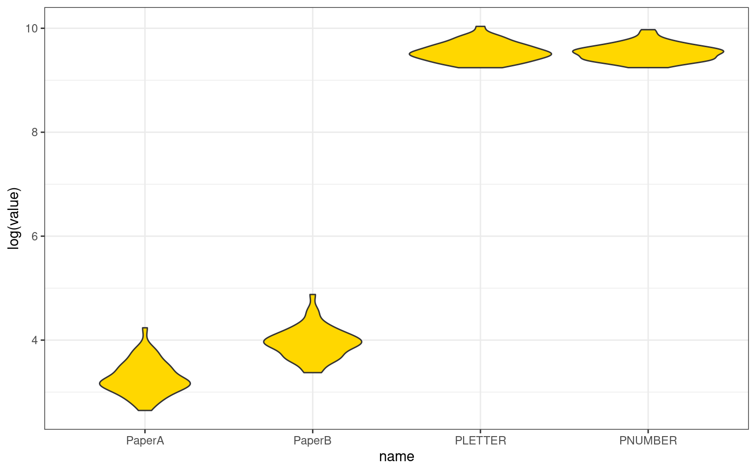
psych::ICC(tmp)Call: psych::ICC(x = tmp)
Intraclass correlation coefficients
type ICC F df1 df2 p lower bound
Single_raters_absolute ICC1 -0.297 0.084 45 138 1.0e+00 -0.3101
Single_random_raters ICC2 0.012 2.468 45 135 3.5e-05 -0.0025
Single_fixed_raters ICC3 0.268 2.468 45 135 3.5e-05 0.1246
Average_raters_absolute ICC1k -10.967 0.084 45 138 1.0e+00 -17.7873
Average_random_raters ICC2k 0.047 2.468 45 135 3.5e-05 -0.0101
Average_fixed_raters ICC3k 0.595 2.468 45 135 3.5e-05 0.3628
upper bound
Single_raters_absolute -0.27
Single_random_raters 0.04
Single_fixed_raters 0.44
Average_raters_absolute -6.18
Average_random_raters 0.14
Average_fixed_raters 0.76
Number of subjects = 46 Number of Judges = 4
See the help file for a discussion of the other 4 McGraw and Wong estimates,The correlation among tests is around .4, except for pnumber/pletter which is .8. So the mean correlation is relatively low, but also the scores are very different–by orders of magnitude. We see a negative ICC value for the absolute ratings ICC1. This does not make sense—ICC is supposed to be a proportion of variance, and cannot be below 0. There is a reason it is negative, for the same reasons that adjusted \(R^2\) and adjusted \(\eta^2\) can be negative, but we probably don’t really care about ICC1 here. These are already very different tests, and we’d be more interested in knowing whether they show a consistent pattern once the absolute scores are factored out. ICC2 values are also close to 0. This allows for randomly-sampled raters on each target, which is also not the case for us. ICC3 is more appropriate–it allows biases among raters, which is sort of what we have. The overall score is positive and less than the average correlation among component measures, but probably representative of the difference between these measures.
With respect to the negative ICC values, ICC is usually estimated with sample mean squares:
The ICC formula becomes:
\((MS_s - MS_e) / (MS_s + (k-1) MS_e + k/n (MS_t - MS_e))\)
Here, \(MS_s\) is subject-related, \(MS_t\) is rater-related, and \(MS_e\) is error-related.
Here, if \(MS_t\) is smaller than \(MS_e\), and \(MS_s\) is small,the denominator can become negative. A negative ICC essentially indicates an ICC of 0, although other measures have been proposed that avoid this issue (see the RWG measure discussed later under inter-rater reliability). The multilevel package also includes a number of other measures of agreement as well, including the rwg measures that avoids the negative values but is not as well developed as the ICC measures. I will provide an example of using several rwg measures below.
Summary of ICC
For a simple test-retest design, correlation is probably OK to use, but ICC has some advantages. If you care about absolute agreement, ICC(1) can be used, but other versions of ICC can factor out absolute ratings values. Furthermore, if you have a pool of raters but nobody rates all targets, ICC can be used. And ICC will give you an overall correspondence value when you have more than just two measures or raters.
The different versions of ICC also make interesting connections to other aspects of psychometrics. Note that ‘single’ ICC attempts to estimate the consistency of a single measurement event, based on multiple measures. Sometimes, the pooled measure is the critical outcome–you might have noisy individual measures but have enough of them that the average score is more robust. Here, the reliability of a single rater is less interesting, and instead you want to measure the reliability of the average of the whole set. This average ICC calculation goes by another name–Cronbach’s \(\alpha\), which is used as a measure of a scale’s `internal consistency’. Rather than thinking about these as multiple independent raters, we think about it as multiple questions on a scale.
Single-measure single-group measures of consistency
Many of the same measures of reliability can be used for inter-rater reliability, although some measures have been proposed that are specific to different response types. We earlier briefly introduced the RWG measure as an alternative to ICC, which is available as part of the `multilevel’ package (James, L. R., Demaree, R. G., & Wolf, G. (1984). Estimating within-group interrater reliability with and without response bias. Journal of Applied Psychology, 69(1), 85–98.).
The multilevel library includes a number of related interrater agreement measures for different situations. The abstract provides a very clear statement of how these might be used, assessing agreement among a single group of judges in regard to a single target: “For example, the group of judges could be editorial consultants, members of an assessment center, or members of a team. The single target could be a manuscript, a lower level manager, or a team. The variable on which the target is judged could be overall publishability in the case of the manuscript, managerial potential for the lower level manager, or a team cooperativeness for the team.”
The RWG measure is mostly a measure of consistency within a single measurement: it does not consider multiple judgments across the same individuals. Its logic is that if we estimate the total potential variability (specified in the ranvar argument), and we look at the observed variability across a group of ratings, the difference between these is the consistency, which is called rwg. the rwg function defaults to assuming you have a 1 to 5 scale with a uniform distribution, which produced a variance of 2. The variance for a uniform rv with A options is $(A^2-1)/12. This can be calculated directly for your own scale, but we can estimate it via simulation as well:
(5^2 - 1)/12[1] 2var(sample(1:5, 1e+05, replace = T))[1] 1.99108Suppose you were using a 1 to 10 scale (it is 8.25)
(10^2 - 1)/12[1] 8.25var(sample(1:10, 1e+07, replace = T))[1] 8.250734The rwg function lets you calculate multiple rwg scores simultaneously, giving a ‘group’ variable and an x variable for scores. We really only need one group thoug. Here is an example with strong consistency:
library(multilevel)
rwg(x = c(3, 3, 3, 4, 3), grpid = c(1, 1, 1, 1, 1))
grpid rwg gsize
1 1 0.9 5Here we have several groups doing ratings on different targets, and the groups have different sizes:
group <- c(1, 1, 1, 1, 1, 2, 2, 2, 3, 3)
values <- c(1, 3, 5, 3, 5, 2, 2, 1, 4, 4)
rwg(x = values, grpid = group)
grpid rwg gsize
1 1 0.0000000 5
2 2 0.8333333 3
3 3 1.0000000 2Here, the first group has no consistency, the second has .83, and the third has 1.0.
Multi-item measures of group consistency.
For RGW, we don’t worry about who is doing the ratings, and concern
ourselves with a single measure. If we have multiple measures we are
taking (i.e., ratings on multiple dimensions), we can make a similar
calculation, and this becomes a measure akin to ICC1, with the advantage
that rwg.j cannot go below 0. The multilevel package has
two functions for this: rwg.j and rwg.lindell.j. rwg.lindell.j uses a
similar calculation but adjusts the score so that it is less likely to
increase as the number of items being judged increase. Both works with
multiple simultaneous ‘groupid’ calculations, but we will look at a
single group rating first. Suppose a panel of judges were rating 4
different gymnasts on a 1 to 5 scale. Here each judge is a row and each
gymnast is a column:
data <- rbind(Russia = c(4, 3, 1, 5), USA = c(5, 3, 5, 5), Japan = c(4, 4, 4, 4))
colnames(data) <- c("A1", "A2", "A3", "A4")
rwg.j(x = data, grpid = rep(1, 3))
grpid rwg.j gsize
1 1 0.6666667 3rwg.j.lindell(x = data, grpid = rep(1, 3)) grpid rwg.lindell gsize
1 1 0.3333333 3This shows reasonable consistency of .666 or .33 for the lindell score. If instead we have a much bigger variability across contestants, but the same variability within each participant, we get the same scores:
data <- rbind(Russia = c(4, 1, 1, 3), USA = c(5, 1, 5, 3), Japan = c(4, 2, 4, 2))
colnames(data) <- c("A1", "A2", "A3", "A4")
rwg.j(x = data, grpid = rep(1, 3))
grpid rwg.j gsize
1 1 0.6666667 3rwg.j.lindell(x = data, grpid = rep(1, 3)) grpid rwg.lindell gsize
1 1 0.3333333 3Measuring Internal Consistency
When your measurement method has multiple –a single set of materials, test-retest validity is difficult to establish because you might get carryover effects. People can learn the materials and be impacted later. Or, for personality-type questionnaires, people may remember their answers and be more consistent than they really should be. Nevertheless, for a scale–a set of questions intended to all measure a coherent construct, we’d like to get a measure of how well they go together, and indirectly a measure of reliability.
There are a number of measures of so-called “Internal consistency”, the most popular among these is Cronbach’s \(\alpha\), which is analogous to the ‘average’ ICC scores. These are sometimes discussed as measuring the average of all possible split-half correlations, but that definition is confusing, because it is not clear whether you are splitting questions and comparing it over people, or splitting people and comparing it over questions. The coefficient \(\alpha\) can be thought of as a measure you would get by dividing your questions into two groups and computing a correlation between them, then repeating this for all possible splits of two groups, adjusted for the total number of items you are measuring. Alternately, as described earlier, it is an adjustment to ICC estimating ICC for the entire set of questions instead of just one.
It is important to recognize that the statistics of consistency make the assumption that there is a single factor underlying the measure, and produce a statistic based on this assumption. Thus, they do not provide strong evidence in favor of a single factor structure when the values are high, but rather measure the consistency based on the assumption that there is a single factor. There are thus ways the statistics can be ‘fooled’. For example, \(\alpha\) goes up as the number of items on the scale go up. In fact, when argueing for researchers to use the Greatest Lower Bound statistic, Sijtsma (2009) argues: ``The only reason to report alpha is that top journals tend to accept articles that use statistical methods that have been around for a long time such as alpha. Reporting alpha in addition to a greater lower bound may be a good strategy to introduce and promote a better reliability estimation practice.’’ It is a good practice to compute a PCA on your data and identify how much variance the first factor accounts for. As a rule of thumb, if the first factor does not account for half of the variance (or ideally more), and if the first factor is multiple times higher than the next largest factor (at least 3x), you probably don’t have a single factor in your items and should try to pick out the subscale you care about.
To examine some alternatives, let’s load a data set using an intelligence/reasoning task similar to Raven’s progressive matrices. These are thought to be a good measure of fluid intelligence. In this data set, we can’t take the results too seriously, because we have fewer people recorded than items on the test. In general, a serious analysis like this should have several hundred observations for a set of 20-50 questions.
library(psych)
library(dplyr)
library(reshape2)
dat.raw <- read.csv("reasoning-dat.csv", header = F)

dat.long <- transmute(dat.raw, sub = V1, prob = V13, correct = V24)
dat <- dcast(dat.long, sub ~ prob, value.var = "correct")
items <- dat[, -1]
Several of the items were correct by everybody, which can cause trouble. These are not predictive of anything. So let’s get rid of them:
items2 <- items[, colMeans(items) < 1]Notice that the measures here are all 0 or 1–whether they got the score correct or not. This will necessarily limit the predictability of any single question.
Now, lets do a PCA to see if we have a single factor. We will look at this in more detail below.
evals <- (eigen(cor(items2))$values)
round(evals/sum(evals), 3)
[1] 0.284 0.146 0.108 0.084 0.073 0.061 0.052 0.049 0.038 0.037 0.026 0.023
[13] 0.013 0.008 0.000 0.000 0.000 0.000 0.000 0.000 0.000 0.000 0.000 0.000
[25] 0.000 0.000 0.000 0.000 0.000 0.000 0.000 0.000 0.000 0.000To start out with this is not promising, because the first factor is only 28% of the variance. This is not too surprising because the Raven’s test contains multiple subscales that have different kiids of difficulty. The first factor is twice as big as the second though, which at least shows a sharp drop-off. Note also that we have relatively few participants(fewer than items), so we could easily get into trouble. We will proceed, but may worry that we have multiple independent factors involved.
Mean or median correlation
One value to consider is the mean or median inter-item correlation.
library(ggplot2)
item.cor <- cor(items2, use = "pairwise.complete")
cor.values <- item.cor[upper.tri(item.cor)]
qplot(cor.values, bins = 50) + annotate(geom = "text", x = 0.5, y = 50, label = paste("Mean:",
    round(mean(cor.values), 3))) + annotate(geom = "text", x = 0.5, y = 55, label = paste("Median:",
    round(median(cor.values), 3))) + xlab("Pairwise correlation")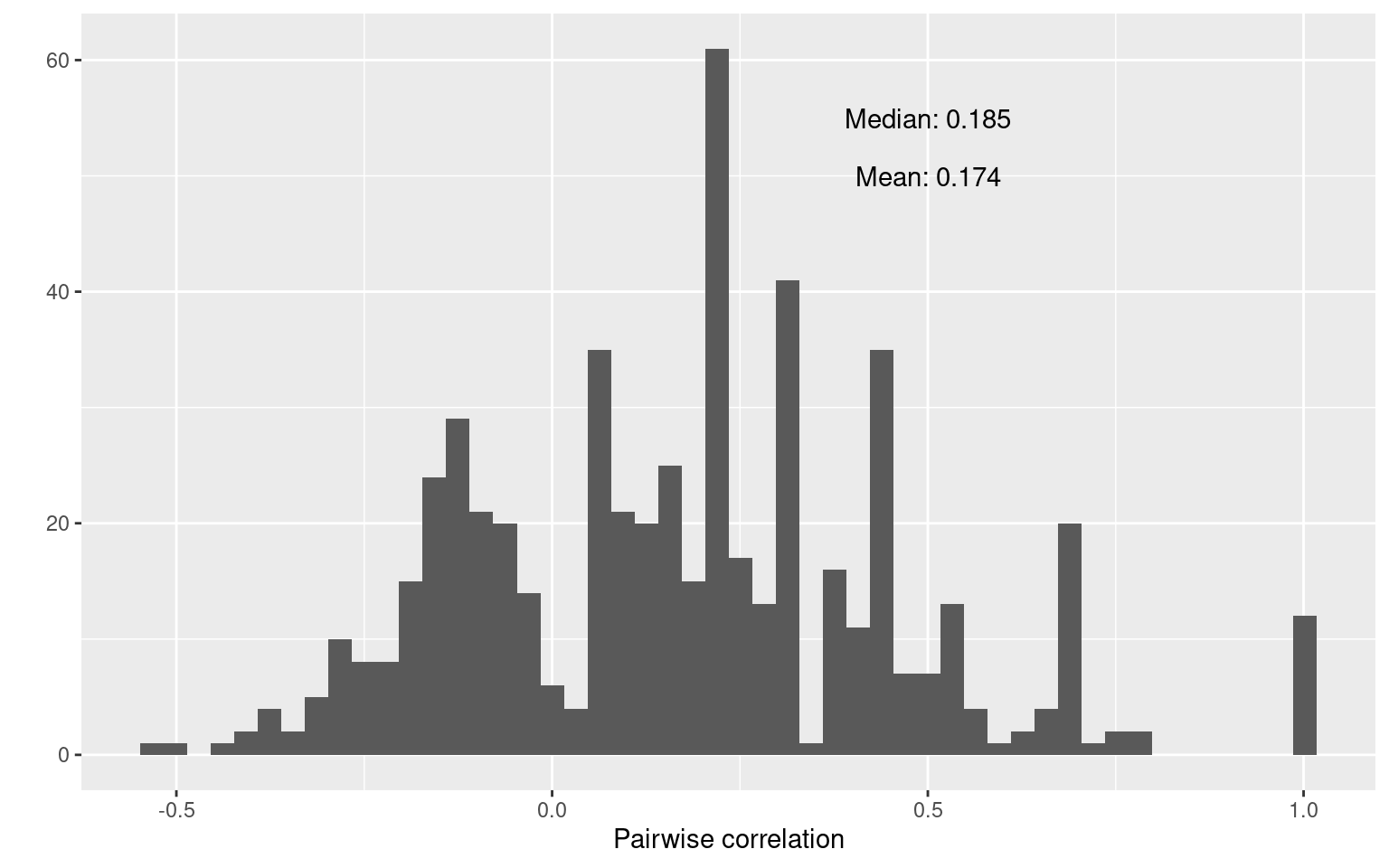
mean(cor.values)[1] 0.17364median(cor.values)[1] 0.1846372This shows that there is fairly weak relationships between items. Many pairs are negatively correlated, and both the mean and median correlations are around .18. On an individual basis, this is not great, but sometimes this as good as we get with single items. Also, see that there are some pairs of items that have a perfect correlation. In our case, this is most likely caused by the small number of participants, but it could also indicate redundancy and might cause problems for some of our methods. In practice, it could also mean that you have asked the same question twice, and one of them could be removed.
Item-total correlation
Another simple measure is to compute the correlation between each item and the total score for each person. In addition to the its ease of interpretation, it can also be used to select variables for inclusion or removal.
library(ggplot2)
library(dplyr)

## Make item total, subtracting out the item score.
itemTotal <- matrix(rep(rowSums(items2), ncol(items2)), ncol = ncol(items2)) - items2

item.cor2 <- diag(cor(items2, itemTotal, use = "pairwise.complete"))
qplot(item.cor2, bins = 20) + annotate(geom = "text", x = 0.5, y = 50, label = paste("Mean:",
    round(mean(item.cor2), 3))) + annotate(geom = "text", x = 0.5, y = 55, label = paste("Median:",
    round(median(item.cor2), 3))) + xlab("Pairwise correlation") + ggtitle("Item-total correlation.")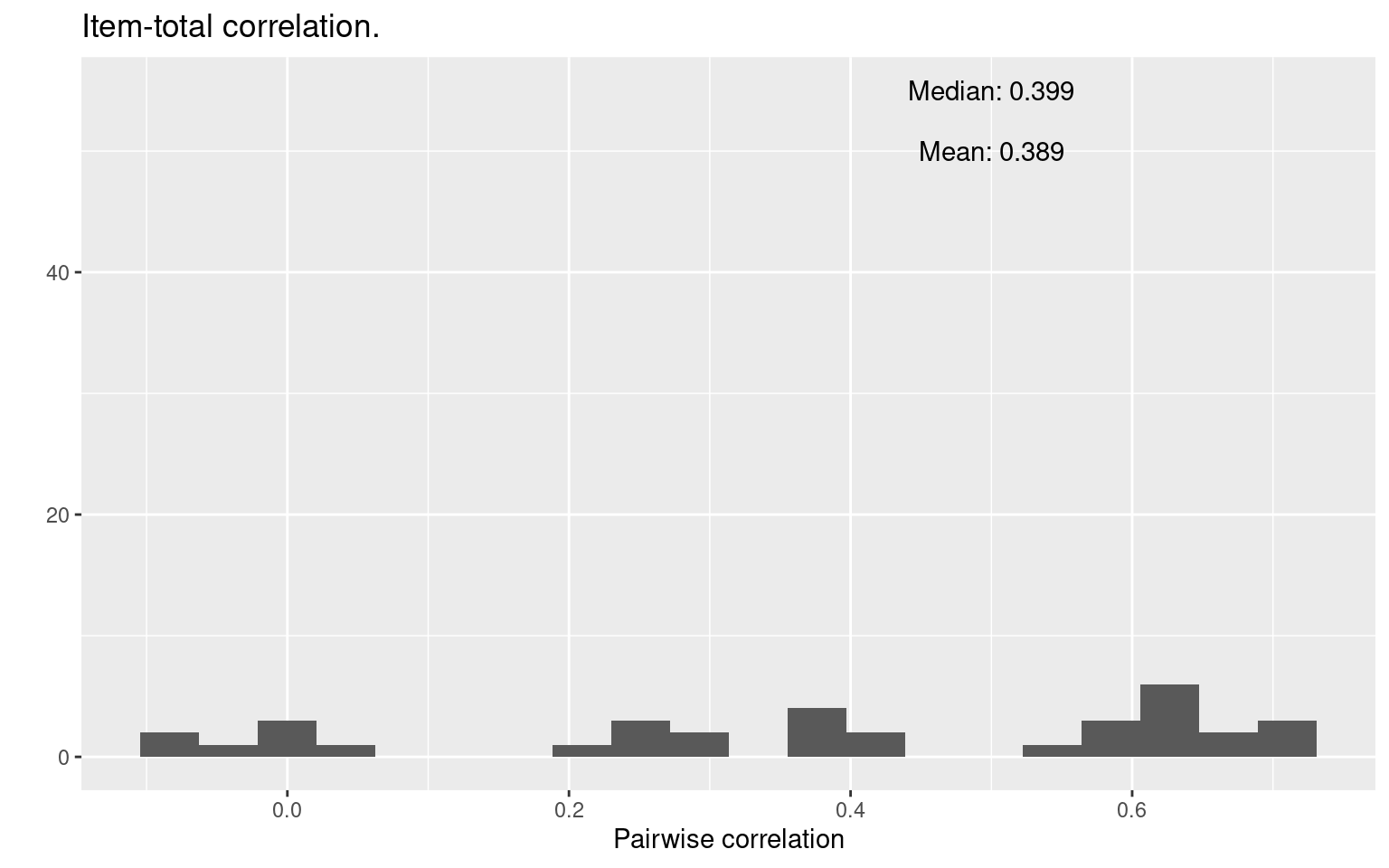
mean(item.cor2)[1] 0.3888878median(item.cor2)[1] 0.3989331This shows how the distribution of scores on each single item correlates (across people) with the total. A high value here means that the question is very representative of the entire set. Possible, it means that you could replace the entire set with that one question, or a small number of questions that are representative of the entire set.
The results here are a bit more reassuring. On average, the correlation between any one item and the total is about 0.4. What’s more, there are a few near 0, and some that are negative, which may indicate that we have “bad” items that we shouldn’t be using. (In this case, it is more likely to stem from the fact that we have a very low number of observations/participants.) Also, about ten questions have item-total correlations around 0.6. Maybe we could make an abbreviated test with just ten questions that is as good as the 40-item test.
Cronbach’s \(\alpha\)
These previous measures are simple heuristics, but several measures have been developed to give a single measure about the coherence of a set of items. The most famous of these is Cronbach’s \(\alpha\) (alpha), which is appropriate for continuous (or at least ordinal)-scale measures, including response time, Likert-style questions, and the like.
Many functions related to psychometrics are available within the package. Other packages including \(\alpha\) include (which also has ICC and a kappa), the library, the package, and probably others.
The package has a function called alpha, which completes computes \(\alpha\) and a more complete reliability analysis, including some of the measures above.
library(psych)
psych::alpha(items2)
Some items ( A3 B2 B5C4D3 C3 D3 D5 ) were negatively correlated with the total scale and
probably should be reversed.
To do this, run the function again with the 'check.keys=TRUE' option
Reliability analysis
Call: psych::alpha(x = items2)

  raw_alpha std.alpha G6(smc) average_r S/N   ase mean   sd median_r
      0.86      0.88    0.85      0.17 7.1 0.049 0.68 0.17     0.18

    95% confidence boundaries
         lower alpha upper
Feldt     0.74  0.86  0.94
Duhachek  0.76  0.86  0.96

 Reliability if an item is dropped:
       raw_alpha std.alpha G6(smc) average_r S/N var.r med.r
A1B3        0.85      0.87    0.84      0.17 6.6 0.078  0.18
A2C3        0.85      0.87    0.84      0.16 6.5 0.080  0.17
A3          0.87      0.88    0.86      0.19 7.5 0.082  0.21
A3B5C4      0.86      0.87    0.85      0.17 6.9 0.087  0.19
A3B5E4      0.86      0.87    0.85      0.17 6.9 0.086  0.18
A3C5D4      0.85      0.87    0.84      0.17 6.6 0.085  0.17
A3C5E4      0.87      0.88    0.86      0.18 7.4 0.083  0.19
A3D5E4      0.85      0.87    0.84      0.17 6.7 0.085  0.17
A4B3D5      0.85      0.87    0.85      0.17 6.8 0.085  0.17
B1E2        0.86      0.87    0.85      0.17 6.9 0.083  0.18
 [ reached 'max' / getOption("max.print") -- omitted 24 rows ]

 Item statistics
        n raw.r std.r  r.cor  r.drop  mean   sd
A1B3   15 0.658 0.725  0.713  0.6326 0.933 0.26
A2C3   15 0.726 0.781  0.775  0.6959 0.867 0.35
A3     15 0.064 0.044 -0.024 -0.0059 0.800 0.41
A3B5C4 15 0.465 0.446  0.411  0.4297 0.067 0.26
A3B5E4 15 0.442 0.436  0.401  0.3922 0.133 0.35
A3C5D4 15 0.706 0.666  0.650  0.6583 0.400 0.51
A3C5E4 15 0.106 0.109  0.046  0.0188 0.467 0.52
A3D5E4 15 0.629 0.609  0.588  0.5730 0.600 0.51
A4B3D5 15 0.610 0.564  0.540  0.5519 0.400 0.51
B1E2   15 0.451 0.497  0.467  0.4018 0.867 0.35
 [ reached 'max' / getOption("max.print") -- omitted 24 rows ]

Non missing response frequency for each item
          0    1 miss
A1B3   0.07 0.93    0
A2C3   0.13 0.87    0
A3     0.20 0.80    0
A3B5C4 0.93 0.07    0
A3B5E4 0.87 0.13    0
A3C5D4 0.60 0.40    0
A3C5E4 0.53 0.47    0
A3D5E4 0.40 0.60    0
A4B3D5 0.60 0.40    0
B1E2   0.13 0.87    0
B2     0.07 0.93    0
B2C5   0.07 0.93    0
B3     0.07 0.93    0
B4     0.27 0.73    0
B4D5E3 0.60 0.40    0
B4E3   0.20 0.80    0
B5     0.60 0.40    0
B5C4D3 0.53 0.47    0
B5C4E3 0.73 0.27    0
B5D4   0.60 0.40    0
C1E4   0.20 0.80    0
C2     0.07 0.93    0
C3     0.13 0.87    0
C3D2   0.33 0.67    0
C4     0.27 0.73    0
 [ reached getOption("max.print") -- omitted 9 rows ]
If you run this with warnings, it will note things like individual items negatively correlated with the total. The results show several results. The ‘raw alpha’ is based on covariances, and the ‘std.alpha’ is based on the correlations. These could differ if you incorporate measures that have very different scales, but should be fairly close if you have all of the same types of questions. These scores turn out to be very good for–actually close to the ``excellent’’ criterion of 0.9. Along with this, it reports G6 –an abbreviation for Guttman’s Lambda (\(\lambda\)). Guttman’s Lambda estimates the amount of variance in each item that can be accounted for by linear regression of all other items. The next column (average_r) computes the average inter-item correlation. This is just an average of the off-diagonals of the correlation matrix. Here, this value is around 0.2. If this were really high, we would need a lot fewer items; because it is relatively low, this means that different questions are not completely predictive of anything else. The final column is a measure of signal-to-noise ratio, which you can read more on in the psych::alpha documentation.
Dropout statistics
Next, it looks at whether any specific items were especially influential, by examining these values if the item were dropped. It shows each of the overall stats for each individual item. These are all make a fairly small change, mostly. This can be accessed directly using alpha(data)$alpha.drop
Item Statistics
Finally, ``Item statistics’’ are shown, which can be accessed directly as alpha(data)$item.stats. These include n, raw.r, std.r, r.cor, r.drop, mean a sd. From the psych help file:
- n number of complete cases for the item
- raw.r The correlation of each item with the total score, not corrected for item overlap.
- std.r The correlation of each item with the total score (not corrected for item overlap) if the items were all standardized
- r.cor Item whole correlation corrected for item overlap and scale reliability
- r.drop Item whole correlation for this item against the scale without this item
Here, we can start thinking about which items are really useful, and which are not, at least to the extent that they intend to measure a common factor. For example, B5C4D3- is actually negatively correlated with the total. This may indicate a good reason to remove the item from the test. However, if there are several factors, it might be a valuable index of another construct.
Examining Eigenfactors and Principle Components (PCA)
Earlier, we stated that \(\alpha\) does not test whether you have a single construct, but rather assumes you do. To be confident in our analysis, we’d like to confirm that all the items fit together. The correlations are somewhat reassuring; but there were a lot of pairwise correlations that were negative and close to 0, which would happen if we had independent factors. To the extent that a specific set of questions are similar, you would expect them to all be correlated with one another. Principle Components analysis attempts to project the correlational structure onto a set of independent vectors using eigen decomposotion. This is related more generally to factor analysis, which will be covered later, and similar questions could be asked in a different way via clustering methods, but the typical approach used by researchers is eigen decomposition, also referred to as principal components analysis.
To the extent that a set of questions coheres, it should be well accounted for by a single factor. PCA identifies a proportion of variance accounted for, and if the proportion of variance for the first dimension is high and, as a rule of thumb, more than 3 times larger than the next, you might argue that the items show a strong coherence.
For a multi-attribute scale (i.e., personality big five) you’d expect multiple factors, but if you isolate just one dimension, you would hope that they can be explained by a single strong factor. We can do a simple factor analysis by doing eigen decomposition of the correlation matrix like this:
cor2 <- cor(items2)
e <- eigen(cor2)
vals <- data.frame(index = 1:length(e$values), values = e$values)
vals$prop <- cumsum(vals$values/sum(vals$values))  #Proportion explained
ggplot(vals, aes(x = index, y = values)) + geom_bar(stat = "identity") + ggtitle("Scree plot of Eigenvalues")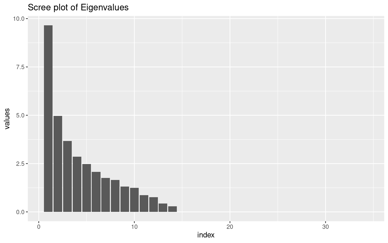
ggplot(vals, aes(x = index, y = prop)) + geom_bar(stat = "identity") + ggtitle("Scree plot of Eigenvalues") +
    ylab("Cumulative Proportion of variance explained")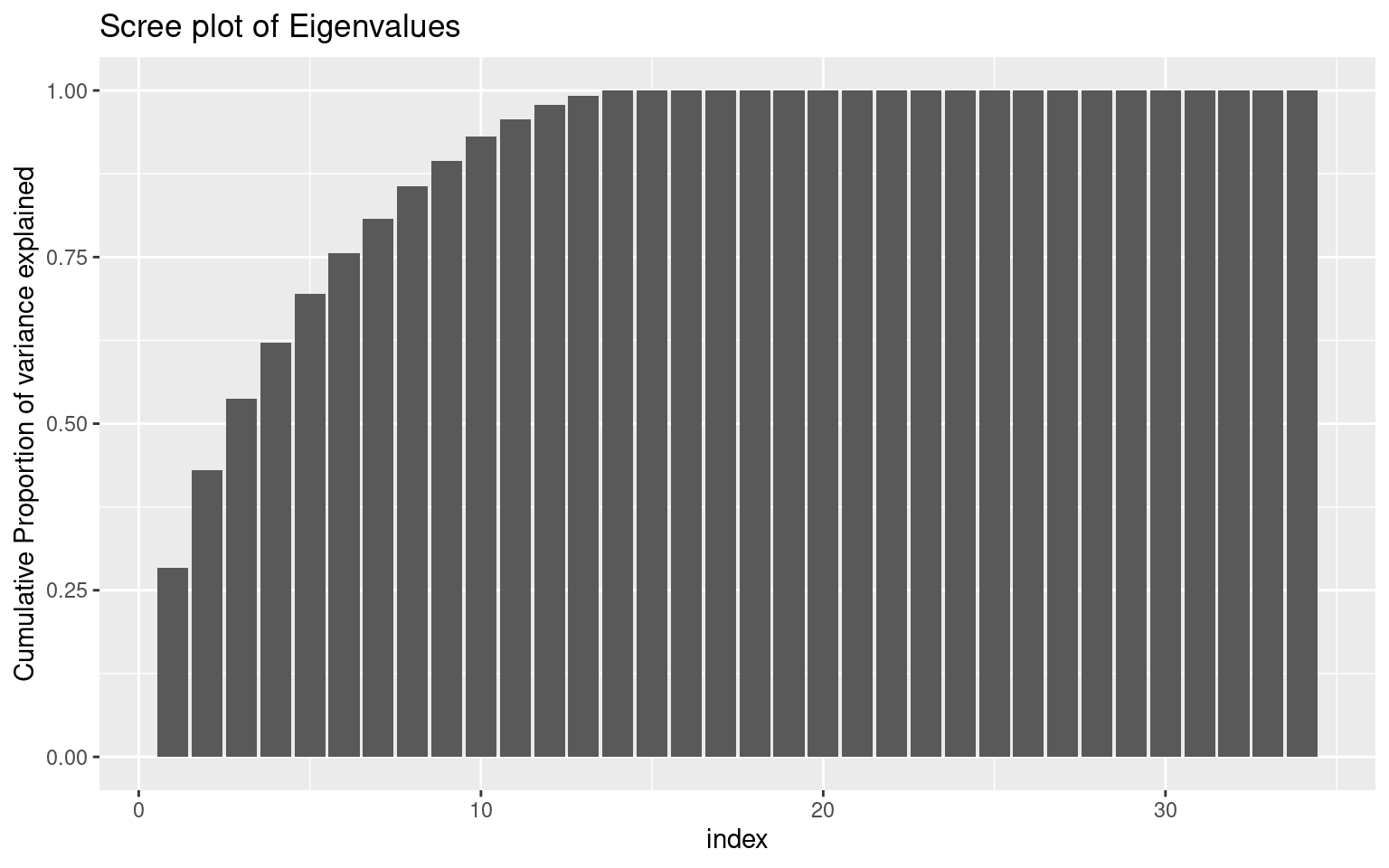
Looking at the ‘scree’ plot, this shows the proportion of variance accounted for by the most to least important dimension. The first dimension is about twice as great as the next, after which it trails off, so this is modestly-strong evidence for a single factor. A basic rule of thumb is that factors with eigenvalues greater than 1.0 are important, suggesting that there are 4-5 factors. The second figure shows cumulative proportion of variance explained (the sum of the eigenvalues is the total variance in the correlation matrix). Here, the results are again not compelling–only 28% of the variance is explained by one factor. These all point to there being multiple constructs that these measures are indexing.
Perhaps we can narrow down the questions to identify a single factor. Looking at the loadings on the first factor, we might look to eliminate values close to 0. It looks like questions 3, 7, 11, 18,23,26,28, and 30 are all relatively small (say less than .07 from 0). What happens if we select just the most strongly associated questions:
(1:34)[abs(e$vectors[, 1]) < 0.07][1] 3 7 11 18 23 26 28 30items3 <- items2[, abs(e$vectors[, 1]) > 0.07]
e2 <- eigen(cor(items3))
vals <- data.frame(index = 1:length(e2$values), values = e2$values)
vals$prop <- cumsum(vals$values/sum(vals$values)) #Proportion explained
ggplot(vals, aes(x = index, y = values)) + geom_bar(stat = "identity") + ggtitle("Scree plot of Eigenvalues")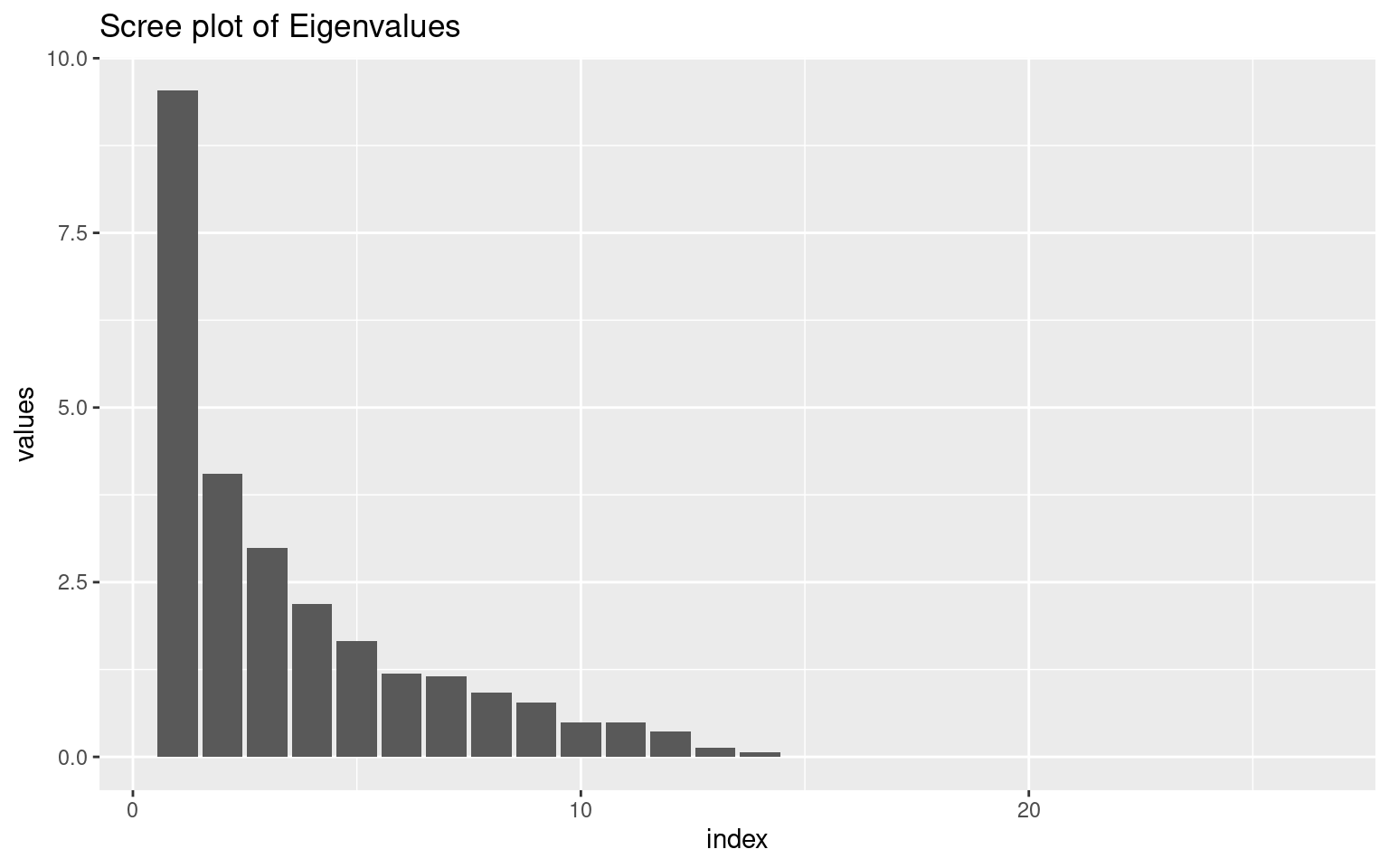
vec1 <- data.frame(index = 1:nrow(e2$vectors), value = e2$vectors[, 1])
ggplot(vec1, aes(x = index, y = value)) + geom_bar(stat = "identity") + ggtitle("Loadings on first eigenvector")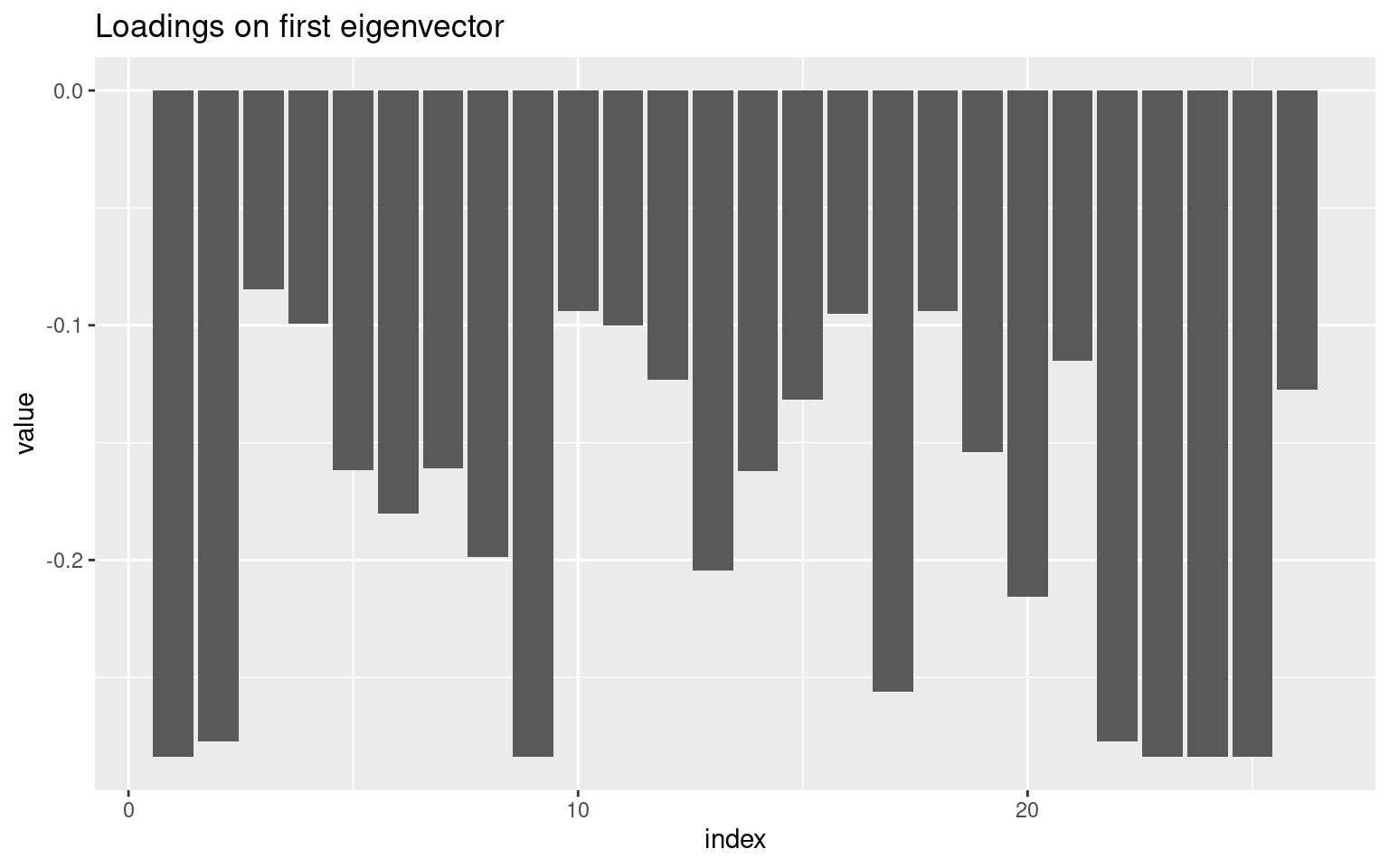
ggplot(vals, aes(x = index, y = prop)) + geom_bar(stat = "identity") + ggtitle("Cumulative Scree plot of Eigenvalues") +
    ylab("Cumulative Proportion of variance explained")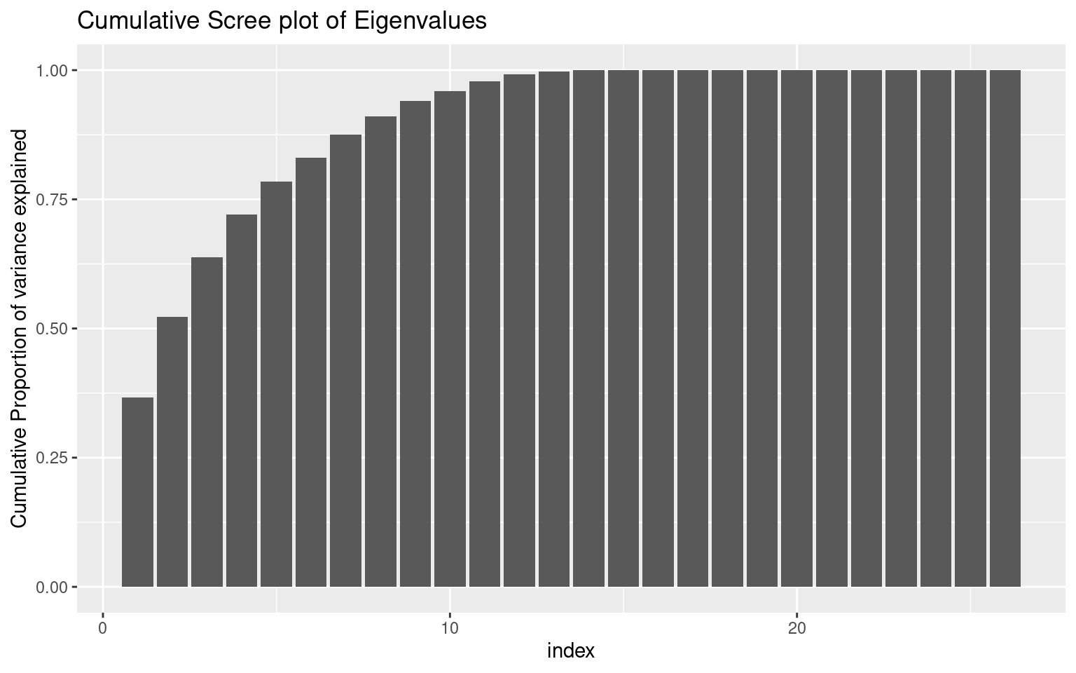
Let’s see what happens when we do the alpha:
alpha(items3)
Reliability analysis
Call: alpha(x = items3)

  raw_alpha std.alpha G6(smc) average_r S/N   ase mean   sd median_r
       0.9      0.92    0.91       0.3  11 0.037 0.66 0.22     0.27

    95% confidence boundaries
         lower alpha upper
Feldt     0.81   0.9  0.96
Duhachek  0.83   0.9  0.97

 Reliability if an item is dropped:
       raw_alpha std.alpha G6(smc) average_r  S/N var.r med.r
A1B3        0.89      0.91    0.91      0.29 10.0 0.065  0.24
A2C3        0.89      0.91    0.91      0.28  9.9 0.068  0.22
A3B5C4      0.90      0.92    0.92      0.31 11.1 0.072  0.29
A3B5E4      0.90      0.92    0.92      0.31 11.0 0.072  0.30
A3C5D4      0.90      0.91    0.92      0.30 10.6 0.072  0.27
A3D5E4      0.90      0.91    0.92      0.30 10.5 0.073  0.24
A4B3D5      0.90      0.91    0.92      0.30 10.6 0.073  0.27
B1E2        0.90      0.91    0.92      0.30 10.6 0.070  0.27
B2C5        0.89      0.91    0.91      0.29 10.0 0.065  0.24
B3          0.90      0.92    0.92      0.31 11.1 0.066  0.29
 [ reached 'max' / getOption("max.print") -- omitted 16 rows ]

 Item statistics
        n raw.r std.r r.cor r.drop  mean   sd
A1B3   15  0.75  0.79  0.76   0.73 0.933 0.26
A2C3   15  0.81  0.85  0.82   0.79 0.867 0.35
A3B5C4 15  0.38  0.36  0.31   0.34 0.067 0.26
A3B5E4 15  0.41  0.40  0.38   0.36 0.133 0.35
A3C5D4 15  0.61  0.56  0.52   0.55 0.400 0.51
A3D5E4 15  0.61  0.59  0.58   0.55 0.600 0.51
A4B3D5 15  0.61  0.57  0.54   0.55 0.400 0.51
B1E2   15  0.52  0.56  0.56   0.48 0.867 0.35
B2C5   15  0.75  0.79  0.76   0.73 0.933 0.26
B3     15  0.36  0.36  0.31   0.32 0.933 0.26
 [ reached 'max' / getOption("max.print") -- omitted 16 rows ]

Non missing response frequency for each item
          0    1 miss
A1B3   0.07 0.93    0
A2C3   0.13 0.87    0
A3B5C4 0.93 0.07    0
A3B5E4 0.87 0.13    0
A3C5D4 0.60 0.40    0
A3D5E4 0.40 0.60    0
A4B3D5 0.60 0.40    0
B1E2   0.13 0.87    0
B2C5   0.07 0.93    0
B3     0.07 0.93    0
B4     0.27 0.73    0
B4D5E3 0.60 0.40    0
B4E3   0.20 0.80    0
B5     0.60 0.40    0
B5C4E3 0.73 0.27    0
B5D4   0.60 0.40    0
C1E4   0.20 0.80    0
C2     0.07 0.93    0
C3D2   0.33 0.67    0
C4     0.27 0.73    0
D1E5   0.40 0.60    0
D4     0.13 0.87    0
E2     0.07 0.93    0
E3     0.07 0.93    0
E4     0.07 0.93    0
 [ reached getOption("max.print") -- omitted 1 row ]
Now, alpha went up, as did all the measures of consistency. This is still weak evidence for a single factor, but also remember we are basing this on a small sample size, and before making any decisions we’d want to collect a lot more data.
Alternate measures of consistency
As discussed before (see Sijtsma, 2009), modern statisticians suggest that \(\alpha\) is fairly useless, and should only be used hand-in-hand with other better measures, including one called glb (greatest lower bound). the psych package provides several alternative measures. Note that for some of these, we don’t have enough observations to do a complete analysis. First, running glb(items3) will compute a set of measures (guttman, tenbarg, glb, and glb.fa).
g <- glb(items3)

g$beta  #worst split-half reliability
[1] 0.6250765g$alpha.pc #estimate of alpha[1] 0.8951595g$glb.max #best alpha[1] 0.9422672g$glb.IC #greatest lower bound using ICLUST clustering[1] 0.9047976g$glb.Km #greatest lower bound using Kmeans clustering[1] 0.8137413g$glb.Fa #greatest lower bound using factor analysis[1] 0.9422672g$r.smc #squared multiple correlation[1] 0.9144583g$tenberge #the first value is alpha$mu0
[1] 0.9167904
$mu1
[1] 0.9286011
$mu2
[1] 0.929218
$mu3
[1] 0.9292724Now, the beta score shows us that possibly our coherence is .47. This converges with our examination of the factors–there might be more than one reasonable factor in the data set.
As a brief test, what happen when our data have two very strong factors in them? Suppose we have 10 items from each of two factors
set.seed(102)
base1 <- rnorm(10) * 3
base2 <- rnorm(10) * 3
people1 <- rnorm(50)
people2 <- rnorm(50)

cor(base1, base2)
[1] -0.1387837These are slightly negatively correlated.
noise <- 0.5

set1 <- outer(people1, base1, "+") + matrix(rnorm(500, sd = noise), nrow = 50)
set2 <- outer(people2, base2, "+") + matrix(rnorm(500, sd = noise), nrow = 50)

data <- as.data.frame(cbind(set1, set2))
image(cor(data))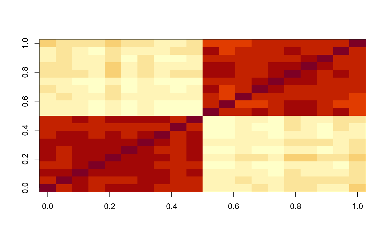
e <- eigen(cor(data))
e$values
[1] 10.02706648 6.93182253 0.41403628 0.34552463 0.30053502 0.27505086
[7] 0.25045743 0.22005759 0.19291691 0.17907262 0.14719890 0.13298576
[13] 0.11112113 0.09858208 0.09272425 0.08485916 0.05798296 0.05511698
[19] 0.04466288 0.03822552alpha(data)
Reliability analysis
Call: alpha(x = data)

  raw_alpha std.alpha G6(smc) average_r S/N   ase mean   sd median_r
      0.95      0.95    0.99      0.47  18 0.013 0.92 0.81     0.26

    95% confidence boundaries
         lower alpha upper
Feldt     0.92  0.95  0.97
Duhachek  0.92  0.95  0.97

 Reliability if an item is dropped:
   raw_alpha std.alpha G6(smc) average_r S/N alpha se var.r med.r
V1      0.94      0.94    0.99      0.47  17    0.014  0.12  0.25
V2      0.94      0.94    0.99      0.47  17    0.014  0.12  0.25
V3      0.94      0.94    0.99      0.47  17    0.014  0.12  0.26
V4      0.94      0.95    0.99      0.48  17    0.014  0.11  0.26
V5      0.94      0.94    0.99      0.47  17    0.014  0.12  0.25
V6      0.94      0.95    0.99      0.47  17    0.014  0.11  0.26
V7      0.94      0.94    0.99      0.47  17    0.014  0.12  0.26
V8      0.94      0.95    0.99      0.48  17    0.013  0.11  0.26
V9      0.94      0.95    0.99      0.48  17    0.013  0.12  0.26
 [ reached 'max' / getOption("max.print") -- omitted 11 rows ]

 Item statistics
     n raw.r std.r r.cor r.drop  mean  sd
V1  50  0.75  0.74  0.73   0.71  0.83 1.2
V2  50  0.76  0.75  0.74   0.72  2.65 1.2
V3  50  0.74  0.72  0.72   0.70 -3.91 1.2
V4  50  0.70  0.69  0.68   0.66  6.21 1.2
V5  50  0.78  0.77  0.77   0.75  3.92 1.2
V6  50  0.70  0.69  0.69   0.67  3.95 1.1
V7  50  0.76  0.75  0.74   0.73  2.92 1.2
V8  50  0.70  0.68  0.68   0.65  1.01 1.2
V9  50  0.69  0.68  0.67   0.65  1.84 1.1
V10 50  0.73  0.71  0.71   0.69  6.07 1.2
[ reached 'max' / getOption("max.print") -- omitted 10 rows ]glb(data)$beta
[1] 0.3090444
$beta.factor
[1] 0.3090444
$alpha.pc
[1] 0.9002699
$glb.max
[1] 0.9658362
$glb.IC
[1] 0.9658362
$glb.Km
[1] 0.3090444
$glb.Fa
[1] 0.9582077
$r.smc
[1] 0.9875206
$tenberge
$tenberge$mu0
[1] 0.947368
$tenberge$mu1
[1] 0.9583356
$tenberge$mu2
[1] 0.9589135
$tenberge$mu3
[1] 0.9589372
$keys
IC1 IC2 ICr1 ICr2 K1 K2 F1 F2 f1 f2
V1 1 0 1 0 0 1 1 0 1 0
V2 1 0 1 0 0 1 0 1 1 0
V3 1 0 1 0 0 1 0 1 1 0
V4 1 0 1 0 0 1 0 1 1 0
V5 1 0 1 0 0 1 0 1 1 0
V6 1 0 0 1 0 1 1 0 1 0
V7 1 0 1 0 0 1 1 0 1 0
[ reached getOption("max.print") -- omitted 13 rows ]glb(set1)$beta
[1] 0.9707496
$beta.factor
[1] NaN
$alpha.pc
[1] 0.883662
$glb.max
[1] 0.9873093
$glb.IC
[1] 0.9805451
$glb.Km
[1] 0.9873093
$glb.Fa
[1] 0.9826313
$r.smc
[1] 0.9823743
$tenberge
$tenberge$mu0
[1] 0.981806
$tenberge$mu1
[1] 0.9818698
$tenberge$mu2
[1] 0.9818825
$tenberge$mu3
[1] 0.981885
$keys
IC1 IC2 ICr1 ICr2 K1 K2 F1 F2 f1 f2
V1 0 1 1 0 1 0 0 1 1 0
V2 0 1 1 0 1 0 0 1 1 0
V3 0 1 1 0 1 0 1 0 1 0
V4 0 1 1 0 1 0 1 0 1 0
V5 1 0 1 0 1 0 0 1 1 0
V6 0 1 0 1 0 1 0 1 1 0
V7 0 1 1 0 0 1 1 0 1 0
[ reached getOption("max.print") -- omitted 3 rows ]Now, we can see that when we don’t have a single factor, we can still get high coefficient alpha, but some of the other measures produced by glb will fail.
Specifying reverse coded elements
Many times, a scale will involve multiple questions, with some reverse coded. That is, a high score on one question (e.g., How much do you like pancakes?) is correlated with a low score on another question (e.g, How much do you hate pancakes?). These are referred to as ‘reverse key’, and the The psych::alpha and glb functions have different ways of handling these.
- psych::alpha will check whether the items are all positively related and give a message if not
psych::alpha(data)
Warning message:
In psych::alpha(dimC) :
  Some items were negatively correlated with the total scale and probably
should be reversed.
To do this, run the function again with the 'check.keys=TRUE' option- psych::alpha will let you specify the names of the variable to reverse code using the keys argument
psych::alpha(data,key=c("q1","q3"))- psych::alpha will also accept a vector of column indices:
psych::alpha(data,key=c(1,3))- pysch::alpha will use its best guess of coding if you use check.keys=T
psych::alpha(data,check.keys=T)- psych::glb will not check automatically and assume that the items are all positive, but provides a $keys output that will help identify different groups
$keys
    IC1 IC2 ICr1 ICr2 K1 K2 F1 F2 f1 f2
Q3    1   0    0    1  0  1  0  1  1  0
Q8    0   1    0    1  0  1  1  0  0  1
Q13   1   0    1    0  1  0  1  0  1  0
Q18   0   1    1    0  0  1  1  0  0  1
Q23   0   1    1    0  1  0  0  1  0  1
Q28   1   0    1    0  1  0  0  1  1  0
Q33   1   0    1    0  0  1  1  0  1  0
Q38   1   0    1    0  0  1  1  0  1  0
Q43 0 1 1 0 1 0 0 1 0 1- psych:splitHalf will accept the check.keys=T argument, which will automatically recode
  psych::splitHalf(dimC,check.keys=T)
Split half reliabilities
Call: psych::splitHalf(r = dimC, check.keys = T)

Maximum split half reliability (lambda 4) =  0.82
Guttman lambda 6                          =  0.77
Average split half reliability            =  0.75
Guttman lambda 3 (alpha)                  =  0.77
Minimum split half reliability  (beta)    =  0.62
Average interitem r =  0.27  with median =  0.26Warning message:
In psych::splitHalf(dimC, check.keys = T) :
Some items were negatively correlated with total scale and were automatically reversed.- psych::glb will not check automatically and assume that the items are all positive, but provides a $keys output that will help identify different groups
$keys
    IC1 IC2 ICr1 ICr2 K1 K2 F1 F2 f1 f2
Q3    1   0    0    1  0  1  0  1  1  0
Q8    0   1    0    1  0  1  1  0  0  1
Q13   1   0    1    0  1  0  1  0  1  0
Q18   0   1    1    0  0  1  1  0  0  1
Q23   0   1    1    0  1  0  0  1  0  1
Q28   1   0    1    0  1  0  0  1  1  0
Q33   1   0    1    0  0  1  1  0  1  0
Q38   1   0    1    0  0  1  1  0  1  0
Q43 0 1 1 0 1 0 0 1 0 1- psych:splitHalf will accept the check.keys=T argument, which will automatically recode and give a warning:
psych::splitHalf(dimC,check.keys=T)
Split half reliabilities
Call: psych::splitHalf(r = dimC, check.keys = T)

Maximum split half reliability (lambda 4) =  0.82
Guttman lambda 6                          =  0.77
Average split half reliability            =  0.75
Guttman lambda 3 (alpha)                  =  0.77
Minimum split half reliability  (beta)    =  0.62
Average interitem r =  0.27  with median =  0.26Warning message:
In psych::splitHalf(dimC, check.keys = T) :
Some items were negatively correlated with total scale and were automatically reversed.- psych::glb will accept a coding vector that is -1/1/0, which differs from psych::alpha:
glb(data,key=c(-1,1,-1,1,1,1))You can use a -1/1 vector in psych::alpha with a coding like this:
psych::alpha(data,key=(1:6)[-1 == c(-1,1,-1,1,1,1)])Exercise.
Load the ability data set from the psych package, and compute coefficient alpha and the other alternative measures.
help(ability)No documentation for 'ability' in specified packages and libraries:
you could try '??ability'Split-half Reliability and correlation
There are two sensible ways in which you might compute a split-half correlation: splitting your items into two bins and correlating across the participants, and splitting participants into two bins and correlating across items. When people discuss split-half reliability, they typically referring to the process of splitting your test into two sub-tests (usually randomly) and finding the correlation. Splitting your participants into two groups and computing the correlation could be used as a way to bootstrap confidence intervals of your correlation coefficient, especially when you are unsure of whether you satisfy assumptions of the tests of statistical inference. Furthermore, if you collect enough data (millions of subjects), you’d expect essentially the same values when splitting your participants into groups. Typically, split-half approaches refer to splitting your items or questions into two groups.
Split-half correlation: splitting questions or items
Oftentimes, there is a natural way to split your questions into two equivalent sub-tests, either for some specific reason (first versus second half) or at random. The rationale for this is often to establish a sort of test-retest reliability within one sample. Some of the psychometric methods will do this for us automatically.
Finally, we can compute reliabilities for split-half comparisons. The splitHalf function will find all split-half comparisons–dividing the test into two sub-tests, computing means, and correlating results. For small numbers of items, it does all possible splits. For more items (> 16), it will sample from the possible splits. Remember that this is sort of what Cronbach’s \(\alpha\) is supposed to be computing anyway. Let’s look at split-half for the first 7 questions. Note that it cannot split 7 evenly, but will instead form all possible splits into two groups and calculate the correlation and range of the two halves and report them. When you have 17 or more items, it samples from the possible splits.
s <- splitHalf(items3[, 1:7])
s
Split half reliabilities
Call: splitHalf(r = items3[, 1:7])
Maximum split half reliability (lambda 4) = 0.88
Guttman lambda 6 = 0.84
Average split half reliability = 0.8
Guttman lambda 3 (alpha) = 0.79
Guttman lambda 2 = 0.8
Minimum split half reliability (beta) = 0.57
Average interitem r = 0.35 with median = 0.33Here, not that the measures for this subset are typically very good (.76+). The beta value–which is the worst-case scenario–is the worst correspondence that was found, and is still somewhat reasonable. What if we had taken 10 items instead?
splitHalf(items3[, 1:10])Split half reliabilities
Call: splitHalf(r = items3[, 1:10])
Maximum split half reliability (lambda 4) = 0.96
Guttman lambda 6 = 0.83
Average split half reliability = 0.82
Guttman lambda 3 (alpha) = 0.82
Guttman lambda 2 = 0.84
Minimum split half reliability (beta) = 0.54
Average interitem r = 0.31 with median = 0.32Notice the the average gets better, but the worst case actually goes down a bit–having more pairings gives more opportunities for a bad correspondence.
You can learn more about the specific statistics reported here using the R documentation–the psych package has very good references and explanations.
Look at the two-factor data set:
glb(data)$beta
[1] 0.3090444
$beta.factor
[1] 0.3090444
$alpha.pc
[1] 0.9002699
$glb.max
[1] 0.9658362
$glb.IC
[1] 0.9658362
$glb.Km
[1] 0.3090444
$glb.Fa
[1] 0.9582077
$r.smc
[1] 0.9875206
$tenberge
$tenberge$mu0
[1] 0.947368
$tenberge$mu1
[1] 0.9583356
$tenberge$mu2
[1] 0.9589135
$tenberge$mu3
[1] 0.9589372
$keys
IC1 IC2 ICr1 ICr2 K1 K2 F1 F2 f1 f2
V1 1 0 1 0 0 1 1 0 1 0
V2 1 0 1 0 0 1 0 1 1 0
V3 1 0 1 0 0 1 0 1 1 0
V4 1 0 1 0 0 1 0 1 1 0
V5 1 0 1 0 0 1 0 1 1 0
V6 1 0 0 1 0 1 1 0 1 0
V7 1 0 1 0 0 1 1 0 1 0
[ reached getOption("max.print") -- omitted 13 rows ]The omega (\(\omega\)) model
Although the glb functions are designed to get around one of the
limitation of Cronbach’s \(\alpha\), it
is not without critics. McDonald (1999)proposed using omega (\(\omega\)) to help determine whether their
scale is primarily a single factor/latent variable. Omega can be
estimated in a number of ways, including one way via PCA and other ways
via structural equation modeling or confirmatory factor analysis. The
basic concept here is that you want to establish that your items on a
scale all load onto a single factor, and that this factor accounts for
an important proportion of variance. Essentially, if we conduct a PCA
and all questions load strongly onto a single factor and that factor
accounts for much of the variance, that is ad hoc evidence for a strong
factor structure. McDonald’s \(\omega_h\) (hierarchical omega) formalizes
this, as a measure of the general factor saturation of a test, and
Revelle et al (2005), the developer of the psych library,
has suggested that \(\omega_h\) is
better than Cronbach’s \(\alpha\) or
another similar measure Revelle’s \(\beta\) (which is worst-case split-half
reliability and reported by glb). The psych library help on
omega provides detailed references and discussion, which you will
probably need to dig deeper into if you plan on using omega, because
there are many options for running and fitting the models and
interpreting them can be tricky. Here, omegah reports a
overall BIC score and 2 factors produces the smallest (most negative)
one, so we will look at that further:
## Total omega. In our case, the output is basically the same as omegah
## omega(data,nfactors=2)omegah(data, nfactors = 2)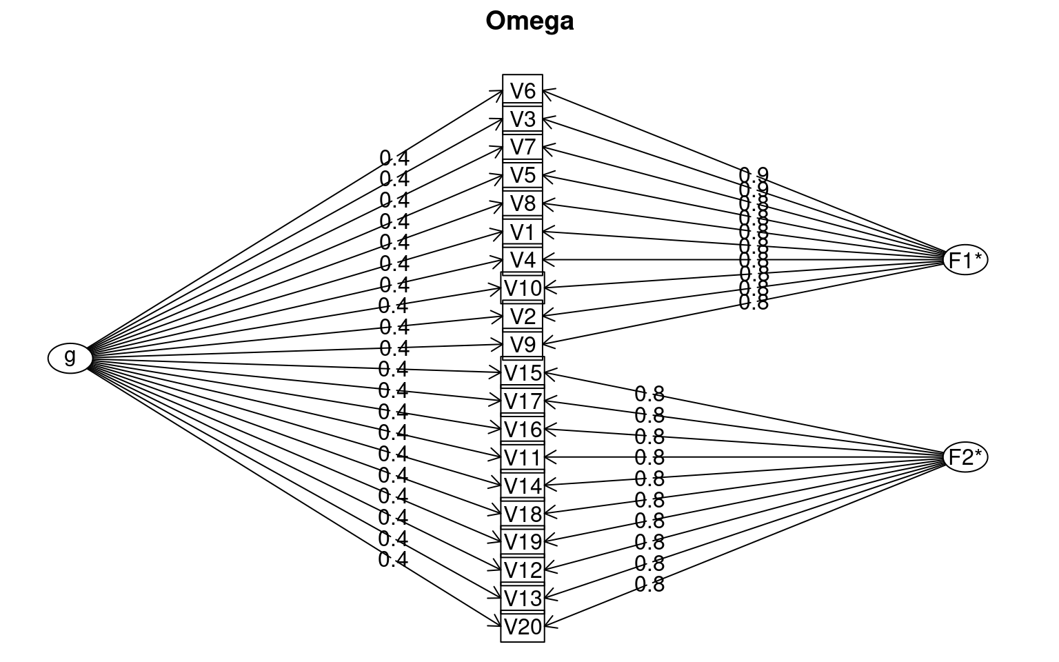
Omega
Call: omegah(m = data, nfactors = 2)
Alpha:                 0.95
G.6:                   0.99
Omega Hierarchical:    0.3
Omega H asymptotic:    0.31
Omega Total            0.98

Schmid Leiman Factor loadings greater than  0.2
       g   F1*   F2*   h2   u2   p2
V1  0.40  0.83       0.85 0.15 0.19
V2  0.41  0.80       0.81 0.19 0.21
V3  0.40  0.85       0.88 0.12 0.18
V4  0.37  0.83       0.83 0.17 0.17
V5  0.42  0.84       0.89 0.11 0.20
V6  0.38  0.86       0.89 0.11 0.16
V7  0.41  0.84       0.88 0.12 0.19
V8  0.37  0.83       0.83 0.17 0.17
V9  0.37  0.80       0.77 0.23 0.17
V10 0.39  0.83       0.83 0.17 0.18
V11 0.37        0.83 0.83 0.17 0.16
V12 0.35        0.79 0.76 0.24 0.16
 [ reached 'max' / getOption("max.print") -- omitted 8 rows ]

With Sums of squares  of:
  g F1* F2*
3.0 6.9 6.7

general/max  0.44   max/min =   1.04
mean percent general =  0.18    with sd =  0.02 and cv of  0.09
Explained Common Variance of the general factor =  0.18

The degrees of freedom are 151  and the fit is  3.54
The number of observations was  50  with Chi Square =  142.12  with prob <  0.69
The root mean square of the residuals is  0.02
The df corrected root mean square of the residuals is  0.02
RMSEA index =  0  and the 10 % confidence intervals are  0 0.055
BIC =  -448.59

Compare this with the adequacy of just a general factor and no group factors
The degrees of freedom for just the general factor are 170  and the fit is  24.43
The number of observations was  50  with Chi Square =  997.57  with prob <  3.7e-117
The root mean square of the residuals is  0.47
The df corrected root mean square of the residuals is  0.5

RMSEA index =  0.311  and the 10 % confidence intervals are  0.296 0.334
BIC =  332.52

Measures of factor score adequacy
                                                  g  F1*  F2*
Correlation of scores with factors             0.55 0.91 0.91
Multiple R square of scores with factors       0.30 0.83 0.83
Minimum correlation of factor score estimates -0.39 0.66 0.66

 Total, General and Subset omega for each subset
                                                 g  F1*  F2*
Omega total for total scores and subscales    0.98 0.98 0.98
Omega general for total scores and subscales  0.30 0.18 0.18
Omega group for total scores and subscales    0.68 0.80 0.80
For this data set, the omega model shows reasonably strong loading
onto a common variance factor g, but also strong loadings of individual
questions onto two additional factors. It provides a chi-squared test
comparing to a general factor-only group and this is highly significant,
indicating the additional factors involving a subgroup of questions are
important. If instead we ran omegah on just the first 10
questions, let’s see what we find:
omegah(data[, 1:10], nfactors = 2)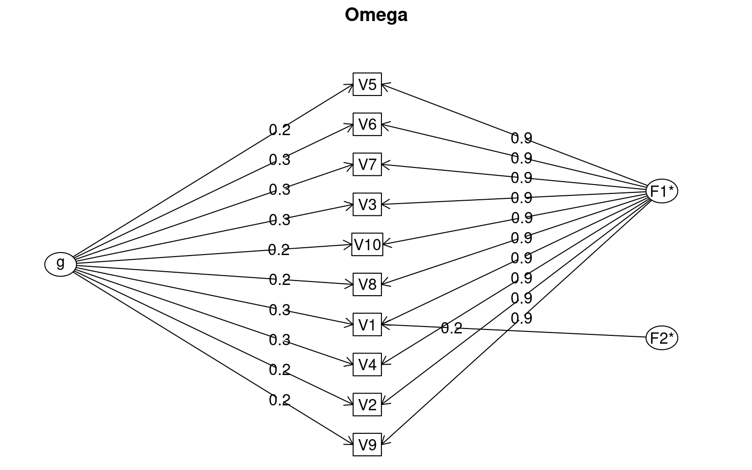
Omega
Call: omegah(m = data[, 1:10], nfactors = 2)
Alpha:                 0.98
G.6:                   0.98
Omega Hierarchical:    0.07
Omega H asymptotic:    0.07
Omega Total            0.98

Schmid Leiman Factor loadings greater than  0.2
       g  F1*   F2*   h2   u2   p2
V1  0.31 0.88  0.24 0.93 0.07 0.11
V2  0.23 0.86       0.80 0.20 0.07
V3  0.28 0.90       0.89 0.11 0.09
V4  0.25 0.87       0.83 0.17 0.08
V5  0.24 0.91       0.88 0.12 0.07
V6  0.27 0.90       0.89 0.11 0.08
V7  0.26 0.90       0.88 0.12 0.08
V8  0.21 0.89       0.86 0.14 0.05
V9  0.20 0.86       0.79 0.21 0.05
V10 0.21 0.89       0.86 0.14 0.05

With Sums of squares  of:
   g  F1*  F2*
0.62 7.85 0.13

general/max  0.08   max/min =   60
mean percent general =  0.07    with sd =  0.02 and cv of  0.27
Explained Common Variance of the general factor =  0.07

The degrees of freedom are 26  and the fit is  0.36
The number of observations was  50  with Chi Square =  15.69  with prob <  0.94
The root mean square of the residuals is  0.01
The df corrected root mean square of the residuals is  0.02
RMSEA index =  0  and the 10 % confidence intervals are  0 0.02
BIC =  -86.03

Compare this with the adequacy of just a general factor and no group factors
The degrees of freedom for just the general factor are 35  and the fit is  12.32
The number of observations was  50  with Chi Square =  544.23  with prob <  1.2e-92
The root mean square of the residuals is  0.78
The df corrected root mean square of the residuals is  0.89

RMSEA index =  0.539  and the 10 % confidence intervals are  0.505 0.586
BIC =  407.31

Measures of factor score adequacy
                                                  g  F1*  F2*
Correlation of scores with factors             0.33 0.96 0.73
Multiple R square of scores with factors       0.11 0.91 0.53
Minimum correlation of factor score estimates -0.78 0.83 0.07

 Total, General and Subset omega for each subset
                                                 g  F1* F2*
Omega total for total scores and subscales    0.98 0.98  NA
Omega general for total scores and subscales  0.07 0.07  NA
Omega group for total scores and subscales    0.91 0.91  NA
Now, the initial BIC score is best for the single factor solution (-110), and that model is not worse than the model with multiple factors. This suggests our first-ten questions fit together well.
Brown-Spearman Prophecy Formula
Typically, the split-half correlation is thought to be biased to under-estimate the true relationship between the two halves. People will sometimes apply the Brown-Spearman prediction formula, which estimates the expected reliability of a test if its length is changed. So, if you have a small test having reliability \(\rho\), then if you were to increase the length of the test by factor \(N\), the new test would have reliability \(\rho^*\).
\[\begin{equation} {\rho}^* =\frac{N{\rho}}{1+(N-1){\rho}} \end{equation}\]For a split-half correlation, you would estimate this as
\[\begin{equation} {\rho}^* =\frac{2{\rho}}{1+{\rho}} \end{equation}\]`
If you complete a split-half correlation of .5, you could adjust this to be \((2\times.5)/(1+.5)= 1/1.5=.6666\). However, especially for small tests and small subject populations, this seems rash, because you probably don’t have a very good estimate of the correlation. We can look at this via simulation:
set.seed(100)
logit <- function(x) {
    1/(1 + 1/exp(x))
}

simulate <- function(numsubs, numitems) {

    submeans <- rnorm(numsubs, sd = 10)
    itemmeans <- rnorm(numitems, sd = 5)

    simdat1 <- (logit(outer(submeans, itemmeans)) > matrix(runif(numsubs * numitems),
        nrow = numsubs, ncol = numitems)) + 0

    simdat2 <- (logit(outer(submeans, itemmeans)) > matrix(runif(numsubs * numitems),
        nrow = numsubs, ncol = numitems)) + 0
    realcor <- cor(rowSums(simdat1), rowSums(simdat2))
    halfcor <- cor(rowSums(simdat1[, 2 * 1:floor(numitems/2)]), rowSums(simdat1[,
        2 * 1:floor(numitems/2) - 1]))
    ## adjusted
    adjusted <- (2 * halfcor)/(1 + halfcor)
    c(realcor, halfcor, adjusted)
}
newvals <- matrix(0, nrow = 100, ncol = 3)
for (i in 1:100) {
    newvals[i, ] <- simulate(1000, 20)
}
colMeans(newvals, na.rm = T)
[1] 0.6518145 0.0422957 -2.7434579newvals[newvals[, 2] < 0, 2] <- NA
newvals[newvals[, 3] < 0, 3] <- NA
cor(newvals, use = "pairwise.complete") [,1] [,2] [,3]
[1,] 1.0000000 0.7379033 0.7481689
[2,] 0.7379033 1.0000000 0.9907501
[3,] 0.7481689 0.9907501 1.0000000head(newvals) [,1] [,2] [,3]
[1,] 0.19215909 NA NA
[2,] 0.19242084 NA NA
[3,] 0.82532920 NA NA
[4,] 0.18154840 NA NA
[5,] 0.20179081 0.008037462 0.01594675
[6,] 0.08867742 0.112542949 0.20231659tmp <- as.data.frame(newvals)
ggpairs(tmp)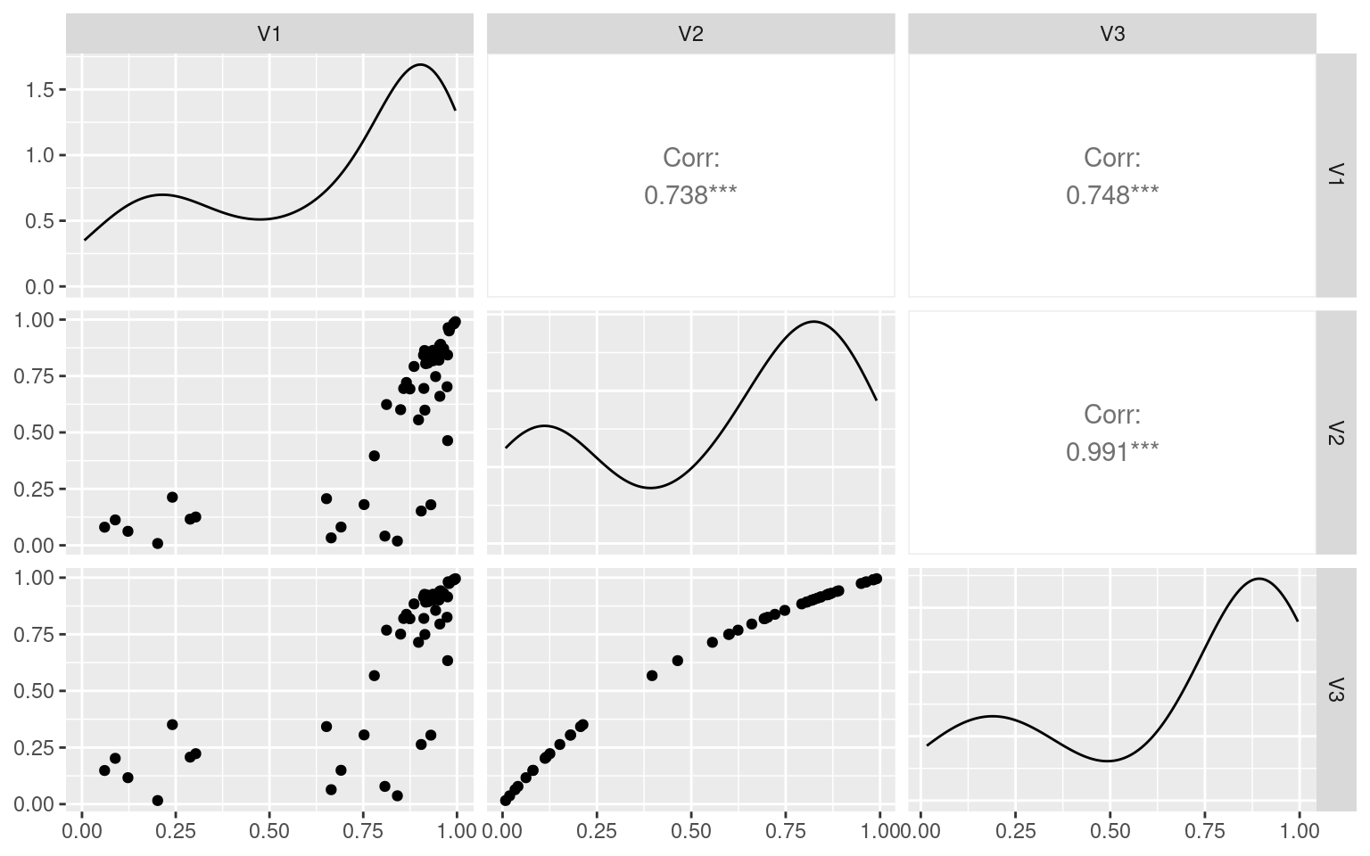
ggplot(tmp, aes(x = V1, y = V3)) + geom_point() + geom_abline(intercept = 0, slope = 1) +
    ggtitle("") + ylab("Estimated reliability") + xlab("True reliability")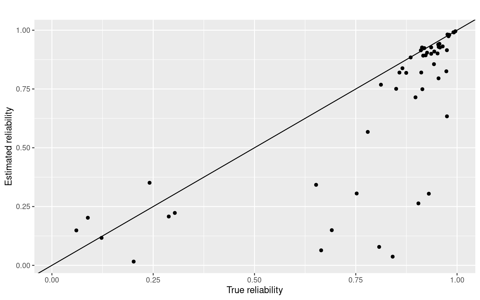
Here, the first number indicates the reliability of the test, built into the simulation. The second number is the estimate for the split-half, and the third number is the adjusted value. If we ignore the cases where the split-half is negative (which happens fairly often), there is a reasonable correlation between the actual estimate of test-retest and the split-half. Even for 1000 participants, in this case.
Categorical Agreement
Cohen’s \(\kappa\) (kappa): agreement of two raters
When you have several nominally-coded sets of scores, correlations won’t work anymore. Instead, we use need another measure of agreement. The standard measure is Cohen’s \(\kappa\). This is most useful for comparing two specific data sets of categorical responses. The library can compute \(\kappa\) using the function.
## courtesy
## http://stackoverflow.com/questions/19233365/how-to-create-a-marimekko-mosaic-plot-in-ggplot2
## see library(ggmosiac) for an alternative that integrates better with ggplot2

makeplot_mosaic <- function(data, x, y, ...) {
    xvar <- deparse(substitute(x))
    yvar <- deparse(substitute(y))
    mydata <- data[c(xvar, yvar)]
    mytable <- table(mydata)
    widths <- c(0, cumsum(apply(mytable, 1, sum)))
    heights <- apply(mytable, 1, function(x) {
        c(0, cumsum(x/sum(x)))
    })

    alldata <- data.frame()
    allnames <- data.frame()
    for (i in 1:nrow(mytable)) {
        for (j in 1:ncol(mytable)) {
            alldata <- rbind(alldata, c(widths[i], widths[i + 1], heights[j, i],
                heights[j + 1, i]))
        }
    }
    colnames(alldata) <- c("xmin", "xmax", "ymin", "ymax")

    alldata[[xvar]] <- rep(dimnames(mytable)[[1]], rep(ncol(mytable), nrow(mytable)))
    alldata[[yvar]] <- rep(dimnames(mytable)[[2]], nrow(mytable))

    ggplot(alldata, aes(xmin = xmin, xmax = xmax, ymin = ymin, ymax = ymax)) + geom_rect(color = "black",
        aes_string(fill = yvar)) + xlab(paste(xvar, "(count)")) + ylab(paste(yvar,
        "(proportion)"))
}
library(psych)
## What if we have high agreement:
a <- sample(1:5, 100, replace = T)
b <- a

cohen.kappa(cbind(a, b))
Call: cohen.kappa1(x = x, w = w, n.obs = n.obs, alpha = alpha, levels = levels)
Cohen Kappa and Weighted Kappa correlation coefficients and confidence boundaries
lower estimate upper
unweighted kappa 1 1 1
weighted kappa 1 1 1
Number of subjects = 100 # replace 10 elements from b
b[sample(1:100, 10)] <- sample(1:5, 10, replace = T)
table(a, b) b
a 1 2 3 4 5
1 9 1 0 0 0
2 0 15 1 0 1
3 0 1 25 1 0
4 1 0 1 23 0
5 0 0 1 0 20tmp <- data.frame(a = a, b = b)
makeplot_mosaic(tmp, a, b)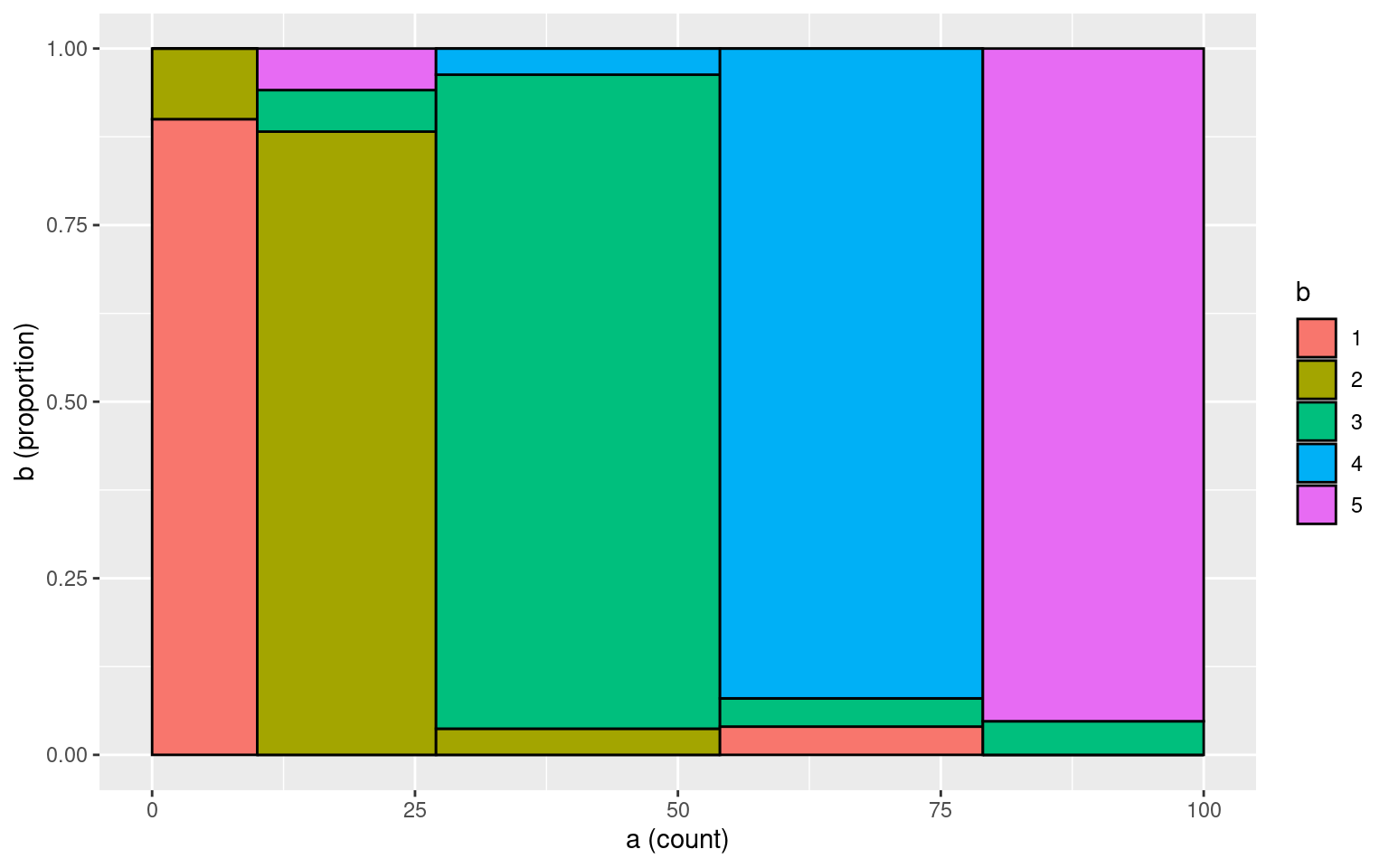
cohen.kappa(cbind(a, b))Call: cohen.kappa1(x = x, w = w, n.obs = n.obs, alpha = alpha, levels = levels)
Cohen Kappa and Weighted Kappa correlation coefficients and confidence boundaries
lower estimate upper
unweighted kappa 0.83 0.90 0.97
weighted kappa 0.91 0.91 0.91
Number of subjects = 100 What if we add more noise:
a <- sample(1:5, 100, replace = T)
b <- a
# replace 50 elements from b
b[sample(1:100, 50)] <- sample(1:5, 50, replace = T)
table(a, b) b
a 1 2 3 4 5
1 17 1 5 1 2
2 2 11 2 4 2
3 0 3 10 0 0
4 0 3 2 15 0
5 3 1 0 4 12# mosaicplot(table(a,b),col=1:5)
tmp <- data.frame(a = a, b = b)
makeplot_mosaic(tmp, a, b)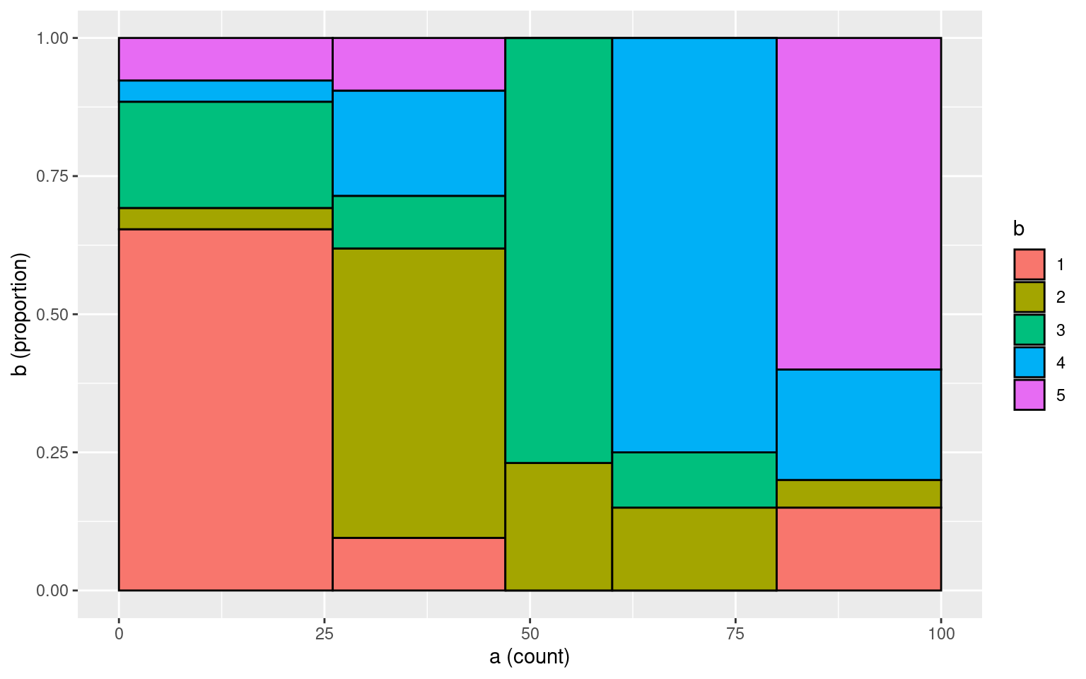
cohen.kappa(cbind(a, b))Call: cohen.kappa1(x = x, w = w, n.obs = n.obs, alpha = alpha, levels = levels)
Cohen Kappa and Weighted Kappa correlation coefficients and confidence boundaries
lower estimate upper
unweighted kappa 0.45 0.56 0.68
weighted kappa 0.40 0.57 0.75
Number of subjects = 100 Sometimes, you might determine that some categories are more similar than others. Thus, you may want to score partial agreement. A weighted version of \(\kappa\) permits this. So, suppose that our five categories represent ways of coding a video for signs of boredom
- rolling eyes
- yawning
- falling asleep
- checking email on phone
- texting on phone
Here, 2 and 3 are sort of similar, as are 4 and 5. Two people coding video might mistake these for one another, and it might be reasonable. So, we can use a weighted \(\kappa\)
a <- sample(1:5, 100, replace = T)
b <- a
b[sample(1:100, 10)] <- sample(1:5, 10, replace = T)

# replace 50 elements from b
b45 <- b == 4 | b == 5
b[b45] <- sample(4:5, sum(b45), replace = T)
b23 <- b == 2 | b == 3
b[b23] <- sample(2:3, sum(b23), replace = T)

weights <- matrix(c(0, 1, 1, 1, 1, 1, 0, 0.5, 1, 1, 1, 0.5, 0, 1, 1, 1, 1, 1, 0,
    0.5, 1, 1, 1, 0.5, 0), nrow = 5, ncol = 5)
table(a, b)
b
a 1 2 3 4 5
1 19 0 0 0 0
2 1 4 12 0 0
3 0 9 10 1 0
4 2 0 1 11 13
5 1 0 0 8 8tmp <- data.frame(a = a, b = b)
makeplot_mosaic(tmp, a, b)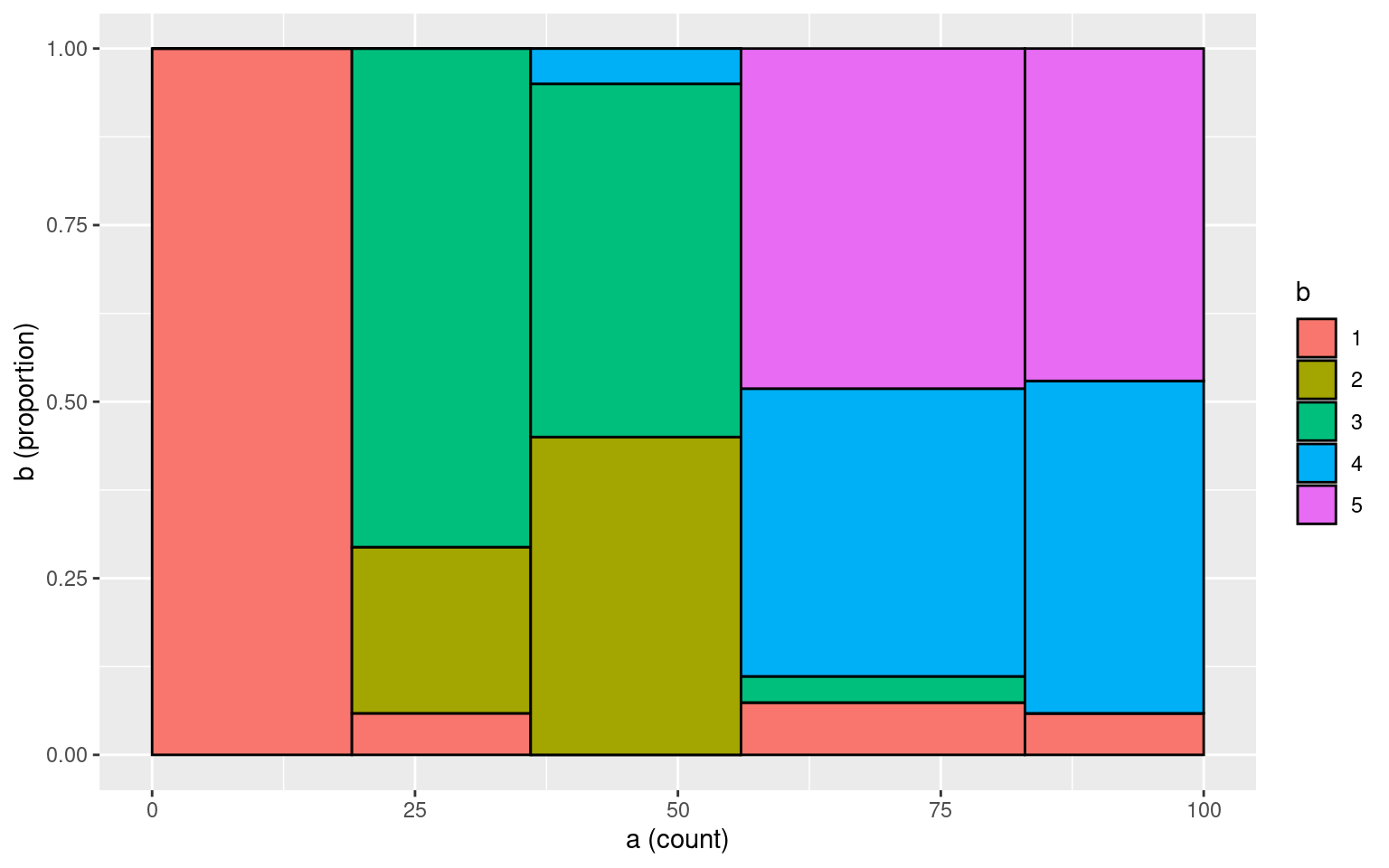
cohen.kappa(cbind(a, b))Call: cohen.kappa1(x = x, w = w, n.obs = n.obs, alpha = alpha, levels = levels)
Cohen Kappa and Weighted Kappa correlation coefficients and confidence boundaries
lower estimate upper
unweighted kappa 0.28 0.4 0.52
weighted kappa 0.70 0.8 0.90
Number of subjects = 100 cohen.kappa(cbind(a, b), weights)Call: cohen.kappa1(x = x, w = w, n.obs = n.obs, alpha = alpha, levels = levels)
Cohen Kappa and Weighted Kappa correlation coefficients and confidence boundaries
lower estimate upper
unweighted kappa 0.28 0.40 0.52
weighted kappa 0.21 0.63 1.00
Number of subjects = 100 Notice how the first value (unweighted) \(\kappa\) does not change when we add weights, but the second weighted \(\kappa\) does change. By default, the weighted version assumes the off-diagonals are ‘’quadratically’ weighted, meaning that the farther apart the ratnigs are, the worse the penalty. This would be appropriate for likert-style ratings, but not for categorical ratings. For numerical/ordinal scales, the documentation claims \(\kappa\) is similar to ICC.
Fleiss’s and Light’s \(\kappa\) (kappa): agreement of multiple raters
The irr library includes kappa2 to
calculate Cohen’s kappa, but also includes two functions to compute
multiple rater categorical agreement: Light’s \(\kappa\) and Fleiss’s \(\kappa\). If we have a third rater c, whose
rating is often the same as a or b’s rating, the data would look like
this:
c <- sample(1:5, size = 100, replace = TRUE)
c[1:40] <- b[1:40]
c[41:80] <- a[41:80]


kappam.light(cbind(a, b, c))
Light's Kappa for m Raters
Subjects = 100
Raters = 3
Kappa = 0.507
z = NaN
p-value = NaN print("---------------")[1] "---------------"kappam.fleiss(cbind(a, b, c)) Fleiss' Kappa for m Raters
Subjects = 100
Raters = 3
Kappa = 0.506
z = 17.4
p-value = 0 These show high agreement across three raters.
Exercise.
Have two people rate the following words into emotional categories: happy, sad, excited, bored, disgusted (HSEBD)
- horse
- potato
- dog
- umbrella
- coffee
- tennis
- butter
- unicorn
- eggs
- books
- rectangle
- water
- soup
- crows
- Canada
- tomato
- nachos
- gravy
- chair
Compute kappa on your pairwise ratings.