Power Analysis
Introduction to Power Analysis
Power analysis is a set of methods for forecasting and understanding the Type-II error rate of an analysis. Most of the time, if we are doing inferential statistics on a data set using a traditional test such as a t-test, we care about the \(p\) value, which estimates the Type I error, or false alarm rate. This reduces the chance of concluding we have a significant difference when one really doesn’t exist. Standard inferential tests ignore Type II errors completely–the chance of failing to find a significant result if it actually does exist. This often makes sense, because so much of experimental science works in the direction of inflating Type I error. For example, if you run an experiment and it fails to reach a p=.05 criterion and thus fails to support your favorite hypothesis, you might collect more observations or subjects and see if that is really the case. It is not hard to see how this can lead to mistaken outcomes.
If you have a null result, you might instead want to know how likely this finding was. It could have failed for several reasons:
- It might have failed because the effect really exists and you messed up something, a measure is unreliable, coded incorrectly, etc.
- It might have failed because the effect does not exist.
- It might have failed because the effect really exists but you did not collect enough data.
If possibility 1 is true, then we need to use our knowledge within the discipline to improve the situation. But how can we distinguish between #2 and #3? One of the tools for this is power analysis, referring to methods to deal with, estimate, or control Type II error. Most resources cite a book by Cohen (1988) as the comprehensive source on this concept:
Cohen, J. (1988). Statistical power analysis for the behavioral sciences (2nd ed.). Hillsdale, NJ: Lawrence Erlbaum.
Challenges for doing power analysis
Power analysis is a forecast. We need some basis for determining how reliable our measures and how large of an effect we expect to have before we can do a legitimate forecast. But if you have a well-understood method, you can often just use your past sample sizes to justify new experiments—if you have a personality questionnaire and found that you needed 500 participants to establish a reliable correlation with behavior, of if you used some interface manipulation and found that 15 participants produced a reliable difference on a usability instrument, you can pin new studies to that sample size and probably be successful.
When you are using a novel procedure, a novel population, a novel instrument/questionnaire, power analysis is the most useful, but also the most difficult to do. The most critical thing you need to assess is the effect size you expect, based on past experiments. Often, you will need to look across a variety of studies and come up with a conservative estimate based on them. For example, for one student’s Master’s thesis, she was testing a new procedure on older adults. Other researchers had tested the older procedure on both young and old adults, and she had previously tested the new procedure on young adults. To forecast the number of participants, she looked across all of these experiments and identified their effect sizes, and conducted power analyses based on a reasonable guess.
I’ve also seen researchers use another strategy—Cohen and others have published interpretations of effect sizes, such as a Cohen’s D of 0.3 is small, a value of .7 is moderate, etc. Sometimes in order to complete a power analysis, researchers simply assert something like “we expect this manipulation to have a small effect size, so we conducted a power analysis using D=.3”. This seems to be barely better than saying “We thought we needed a sample size of 50 to find the result, so we used a sample size of 50”.
The Risks and costs of using underpowered (and overpowered) studies
There are a number of direct and indirect risks and costs that could occur if you don’t do a power analysis. Some include:
Using a study that is underpowered means you are wasting resources. If you know you have a 20% chance of finding a result if it really existed, you are really just gambling, not conducting a legitimate test.
If you are actually right about the effect size and you run an underpowered study, then if you find a result it is more likely to have arisen because of random chance or other mistakes.
If you fail to find a significant result, you might overweight the null hypothesis.
A smaller sample size will include more variability in means, and especially if you conduct multiple tests, you might be more likely to find spurious results
You may be tempted to conduct several small underpowered studies rather than one larger correctly powered study. This will escalate the chance of a false positive, and so it will subvert the p-value calculations and is a form of p-hacking. Furthermore, it is exacerbated by the fact that non-significant results rarely get published.
If you don’t plan the experiment upfront, you also subvert the p-value calculations, because you essentially allow yourself a stopping rule–collect observations until I either find the result or run out of time/money/patience.
When you publish a paper, it is becoming more common to report power analysis you did because this helps the reader understand whether the results (especially the null results) were likely to have been found in the study being reported. If your power analysis showed you needed 100 participants to produce a result, but you only collected 25, and you did not find the result, there is really very little you can conclude from the study.
If you use too large of a sample size, you are obviously also wasting resources. In addition, you are more likely to detect small meaningless differences as significant. You should target an effect size that you think is meaningful. For example, you might want to know whether the fontface, color, or font size of labeling or instructions has an impact on the usability of a device or advertisement. In some cases, it might be really easy to collect thousands of respondents, which would mean that you could detect a statistically significant difference that is very small. It is almost certainly true that there is likely to be some true difference, but you need to think about what is the reasonably smallest practical difference you are interested in. You might end up determining dark blue instruction fonts lead to 1% better understanding than black, and that this is a statistically significant difference, but hardly meaningful.
Illustrating the logic of power analysis for a two-sample t-test
Suppose we have a phenomena with true but small between-group difference. We collect 100 observations in each of two groups.
library(ggplot2)
set.seed(100)
groupA <- rnorm(100, mean = 10)
groupB <- rnorm(100, mean = 10.5)
t.test(groupA, groupB)
    Welch Two Sample t-test

data:  groupA and groupB
t = -3.926, df = 186.92, p-value = 0.0001213
alternative hypothesis: true difference in means is not equal to 0
95 percent confidence interval:
 -0.7636017 -0.2528548
sample estimates:
mean of x mean of y
 10.00291  10.51114
This effect is very strong, and we can detect in with a large experiment. But suppose collecting data is very expensive, and you could only collect 10 in each group:
t.test(groupA[1:10], groupB[1:10])
    Welch Two Sample t-test

data:  groupA[1:10] and groupB[1:10]
t = -1.3939, df = 14.98, p-value = 0.1837
alternative hypothesis: true difference in means is not equal to 0
95 percent confidence interval:
 -1.1918662  0.2494373
sample estimates:
mean of x mean of y
 9.982043 10.453257
So, this test was not statistically significant; even though the
means were actually very close to the true means of the groups. We would
like to know how likely we would have been to find a null effect in an
experiment this size. We can use the pwr library to do
this. All of the pwr functions take at least four
arguments:
- sample size
- effect size
- significant level (p-value; Type-I error rate)
- power (1 minus Type-II error rate)
Estimating power
Some of the specific power functions will also take other arguments,
such as whether the test is one-sided or two-sided. In this case, since
we conducted the experiment already, let’s try to estimate the power. To
do so, we need to compute the effect size. In the case of a t-test, we
use Cohen’s d–the standardized difference between means, or \(\delta/sd\). The pwr library
by Stephane Champely will do many power calculations for you, although
there are many on-line tools available and other custom software
available in other packages.
d <- abs(mean(groupA[1:10]) - mean(groupB[1:10]))/sd(c(groupA[1:10] - mean(groupA[1:10]),
    groupB[1:10] - mean(groupB[1:10])))
library(pwr)
pwr.t2n.test(n1 = 10, n2 = 10, d, sig.level = 0.05, power = NULL)
     t test power calculation

             n1 = 10
             n2 = 10
              d = 0.6404344
      sig.level = 0.05
          power = 0.2734475
    alternative = two.sided
test <- pwr.t.test(n = 10, d, sig.level = 0.05)
test
     Two-sample t test power calculation

              n = 10
              d = 0.6404344
      sig.level = 0.05
          power = 0.2734475
    alternative = two.sided

NOTE: n is number in *each* group
## plotting the test shows trade-off of sample size to power:
plot(test)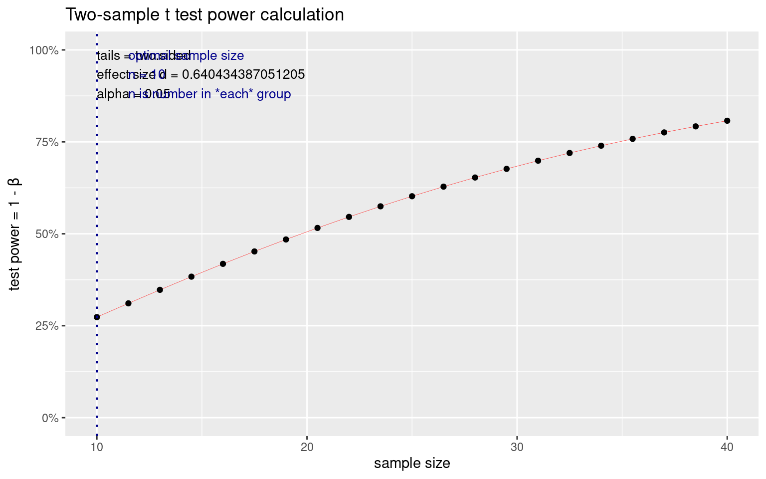
We can specifiy the power analysis with either of these functions, where n is the number in each group. Here, we can see that with a .05 signiificance level and the results we found, we’d expect a power of .25. This is a 75% chance of making a Type-II error. That is, in the experiment we ran, 75% percent of the time that there was a true difference of the size we measured, we’d expect that we would fail to find it.
Estimating sample size
We might decide that we need to run another experiment based on this one. Supposing we have the same effect size, how many subjects would we need? The rule of thumb for power analysis is typically that we seek to have a test with power of 0.8–we want an 80% chance of finding the effect if it really is there, with a p-value of .05–a 5% chance of finding an effect that is not there. The pwr.t2n.test won’t work well, because it lets N1 and N2 differ, so we ca only use pwr.t.test:
test <- pwr.t.test(d = d, sig.level = 0.05, power = 0.8)
test
     Two-sample t test power calculation

              n = 39.25641
              d = 0.6404344
      sig.level = 0.05
          power = 0.8
    alternative = two.sided

NOTE: n is number in *each* groupplot(test)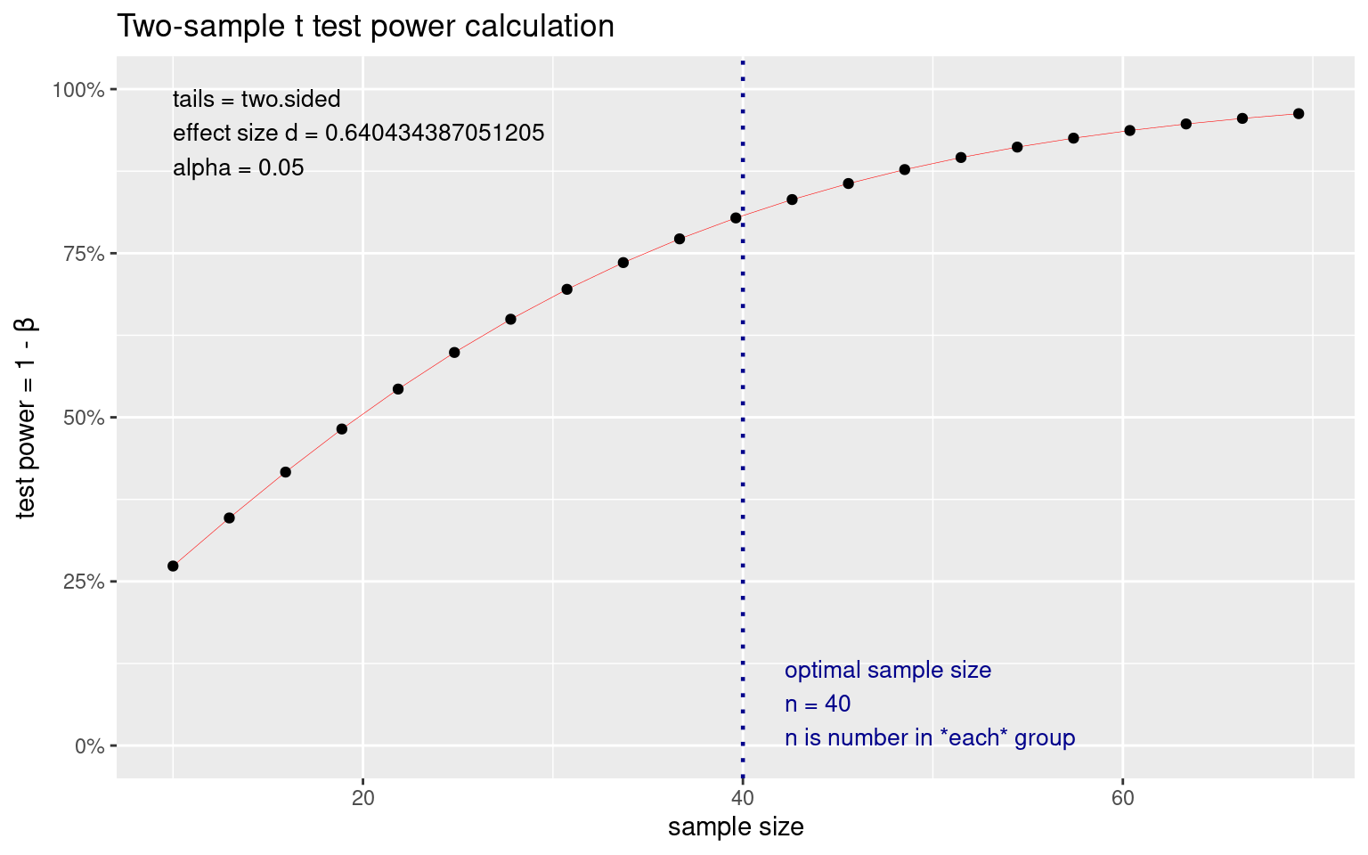
This suggests that we really need to collect 44 participants in each group to stand a good chance of finding the result. If this study cost $200 per subject, we have just determined that it will cost $9,000 to run the study, which may be out of our budget and thus not worthing doing. Instead, we might take a look at our measures and try to find ways to produce larger effect sizes; maybe via a within-subject design or with a more reliable set of measures (like with double the number of observations or items).
Estimating Effect size
So we have determined that our experiment won’t work. Suppose that we have enough money to run 20 subjects in each group in our new experiments.
test <- pwr.t.test(sig.level = 0.05, n = 20, power = 0.8)
test
     Two-sample t test power calculation

              n = 20
              d = 0.9091587
      sig.level = 0.05
          power = 0.8
    alternative = two.sided

NOTE: n is number in *each* groupplot(test)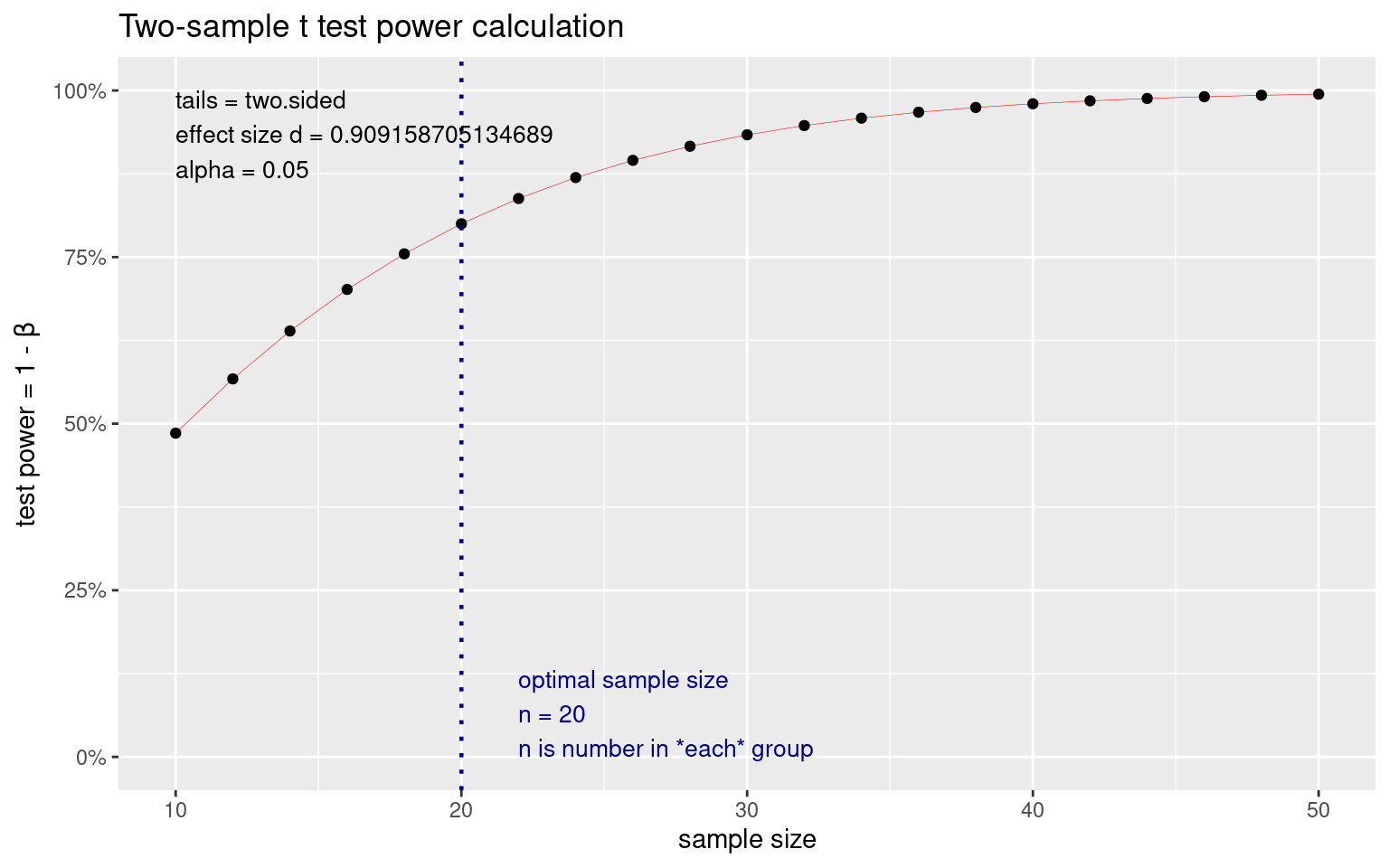
This is good news. If we can find a way to cut the variability of our test roughly in half and increase the effect size to .9, we would be able to find the effect with 20 participants.
Estimating p-value
Another way to look at it is to ask about the type-I error rate fixing the other parameters. This might be more appropriate in practical non-scientific settings, where you need to conduct a study to make a decision, but your managers have determined that the amount you can spend on the test is limited because it has to be paid for by the amount you expect to benefit by from choosing the better design (interface, method, device, product, food, etc.). This would not be acceptable in a scientific context, but it might be acceptable for A/B testing of web sites or products.
test <- pwr.t.test(n = 20, d = 0.6, power = 0.8, sig.level = NULL)

test
     Two-sample t test power calculation

              n = 20
              d = 0.6
      sig.level = 0.2946697
          power = 0.8
    alternative = two.sided

NOTE: n is number in *each* groupplot(test)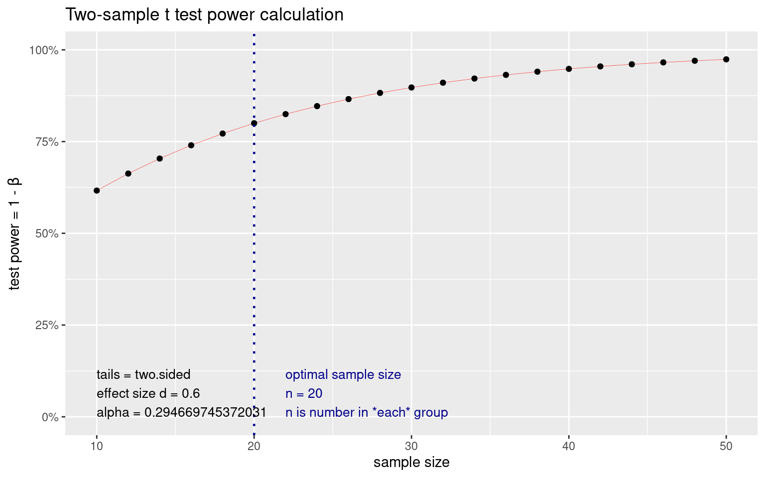
Here, we can see that the significance level is .29, which is actually about the same \((1-power)\). If we split the difference, we can see they are about equal:
test <- pwr.t.test(n = 20, d = 0.6, power = 0.76, sig.level = NULL)
test
     Two-sample t test power calculation

              n = 20
              d = 0.6
      sig.level = 0.2391074
          power = 0.76
    alternative = two.sided

NOTE: n is number in *each* groupplot(test)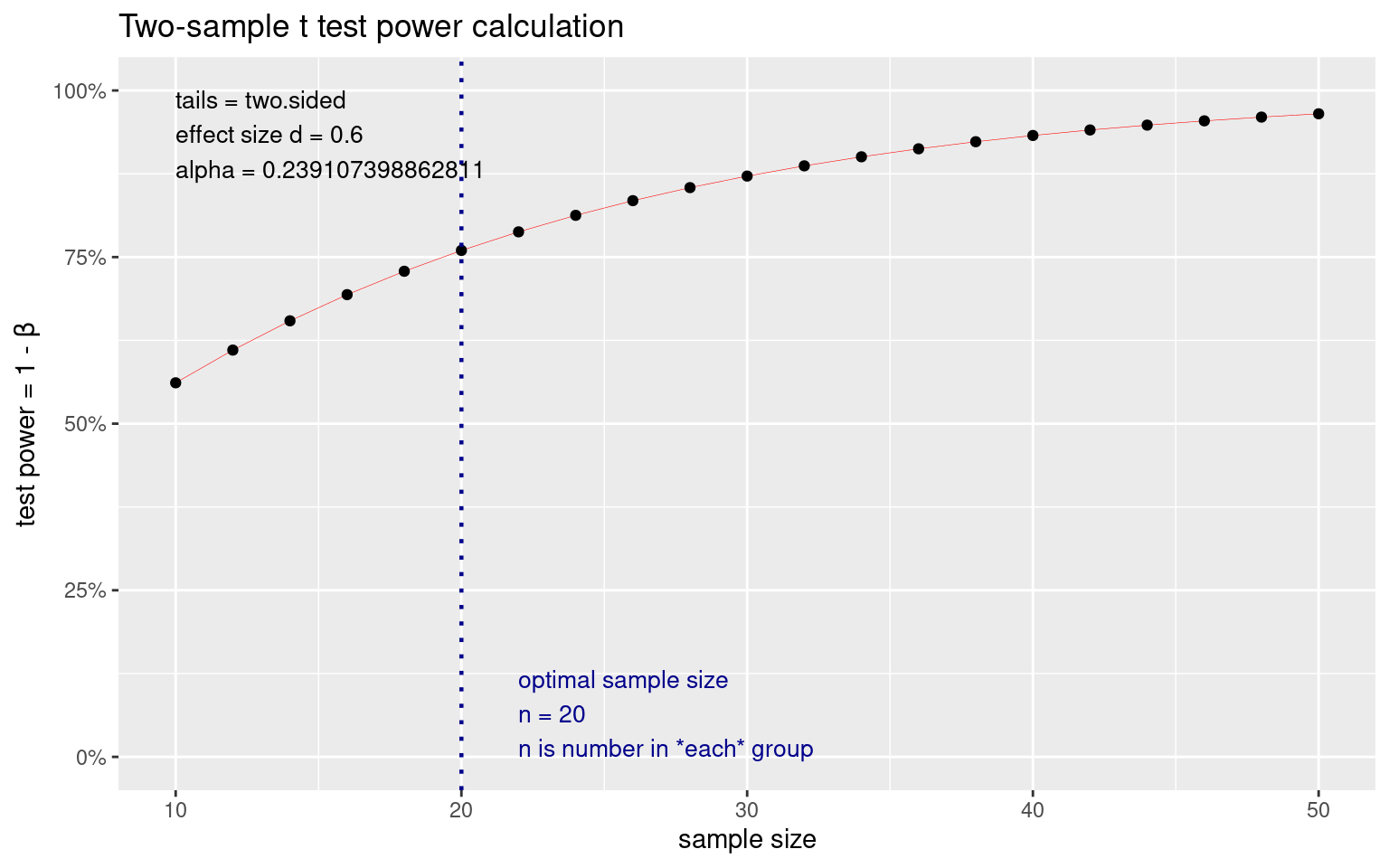
So, if we know we have an effect size of .6 and can only afford to test 20 people in each group, then by picking a p-value of .24, we have a power of .76. Here Type I and Type II error rates are essentially equal. This means that if one option is better, we will see it 3/4 of the time and if the options don’t differ, we will see no difference 3/4 of the time. If you could further quantify the costs and benefits of each type of error, you could make other decisions that will optimize the test design.
Overview of power calculation for particular tests within pwr.
Power can be computed for a number of tests
pwr-package Basic Functions for Power Analysis pwr
cohen.ES    Conventional effects size
ES.h    Effect s ize calculation for proportions
ES.w1   Effect size calculation in the chi-squared test for goodness of fit
ES.w2   Effect size calculation in the chi-squared test for association
plot.power.htest    Plot diagram of sample size vs. test power
pwr Basic Functions for Power Analysis pwr
pwr.2p.test Power calculation for two proportions (same sample sizes)
pwr.2p2n.test   Power calculation for two proportions (different sample sizes)
pwr.anova.test  Power calculations for balanced one-way analysis of variance tests
pwr.chisq.test  power calculations for chi-squared tests
pwr.f2.test Power calculations for the general linear model
pwr.norm.test   Power calculations for the mean of a normal distribution (known variance)
pwr.p.test  Power calculations for proportion tests (one sample)
pwr.r.test  Power calculations for correlation test
pwr.t.test  Power calculations for t-tests of means (one sample, two samples and paired samples)
pwr.t2n.test    Power calculations for two samples (different sizes) t-tests of means
Power for t-tests
The above examples show how to calculate power fo independent-sample t-tests, either with equal or unequal numbers of groups. If you have a paired-samples or one-sample t-tests, you can specify the type argument to make those calculations:
## Calculate power of a two-measure within-subject test
pwr.t.test(n = 50, d = 0.4, sig.level = 0.05, type = "paired")
     Paired t test power calculation

              n = 50
              d = 0.4
      sig.level = 0.05
          power = 0.7917872
    alternative = two.sided

NOTE: n is number of *pairs*pwr.t.test(n = 50, d = 0.4, sig.level = 0.05, type = "two.sample")
     Two-sample t test power calculation

              n = 50
              d = 0.4
      sig.level = 0.05
          power = 0.5081857
    alternative = two.sided

NOTE: n is number in *each* group
## Calcualte power of one-sample test--determine whether the mean is different
## from 0.
pwr.t.test(n = 50, d = 0.4, sig.level = 0.05, type = "one.sample")
     One-sample t test power calculation

              n = 50
              d = 0.4
      sig.level = 0.05
          power = 0.7917872
    alternative = two.sided
Power of correlations
For correlations, the \(R\) value IS the effect size (or more properly \(R^2\), the total proportion of variance accounted for). In many personality experiments, inter-scale correlations will have a maximum correlation of about 0.3. How many participants would we need to measure if this were true?
test <- pwr.r.test(n = NULL, r = 0.3, sig.level = 0.05, power = 0.8)
test
     approximate correlation power calculation (arctangh transformation)

              n = 84.07364
              r = 0.3
      sig.level = 0.05
          power = 0.8
alternative = two.sidedplot(test)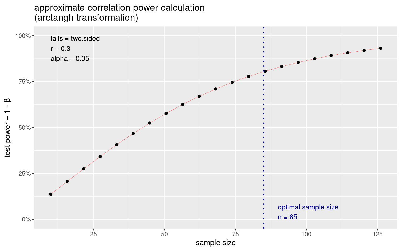
This is a lot larger than many people’s intuition. The plot shows that with if we had collected only 50 participants, the power dips to close to .5. What if we expect a slightly smaller correlation of 0.25?
test <- pwr.r.test(n = NULL, r = 0.25, sig.level = 0.05, power = 0.8)
test
     approximate correlation power calculation (arctangh transformation)

              n = 122.4466
              r = 0.25
      sig.level = 0.05
          power = 0.8
    alternative = two.sided
Suppose we had a study of 1000 participants and found a correlation of about +.05, which was not significant. What was the power to detect true differences of this size in our experiment?
set.seed(100)
x <- runif(1000)
y <- x + runif(1000) * 50
cor.test(x, y)
    Pearson's product-moment correlation

data:  x and y
t = 1.6173, df = 998, p-value = 0.1061
alternative hypothesis: true correlation is not equal to 0
95 percent confidence interval:
 -0.01089842  0.11276487
sample estimates:
       cor
0.05112921
test <- pwr.r.test(n = 1000, sig.level = 0.106, power = NULL, r = 0.05)
test
     approximate correlation power calculation (arctangh transformation)

              n = 1000
              r = 0.05
      sig.level = 0.106
          power = 0.48653
alternative = two.sidedplot(test)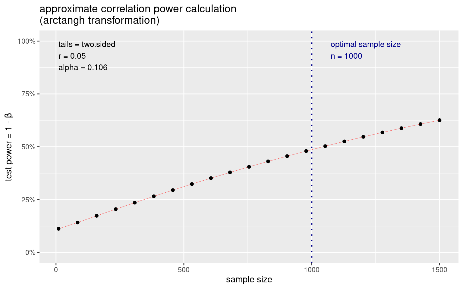
Power in One-way ANOVA and F tests
For general ANOVA tests that we might use in regression or ANOVA, the pwr.f2.test or pwr.anova.test are used.
The effect size these tests use is \(f^2\), where \(f^2 = {{R^2}\over {1-R^2}}\) (don’t be confused with the actual \(F\) value.) To use this, we need to know the degrees of freedom associated with the test.
Notice that if \(R^2\) is very high, you \(f^2\) will be very high. If \(R^2\)=.5, \(f^2=1.0\). The pwr library includes some lookup functions to help you judge what might be considered a large versus small effect size:
cohen.ES(test = "f2", size = "small")
     Conventional effect size from Cohen (1982)

           test = f2
           size = small
effect.size = 0.02cohen.ES(test = "f2", size = "medium")
     Conventional effect size from Cohen (1982)

           test = f2
           size = medium
effect.size = 0.15cohen.ES(test = "f2", size = "large")
     Conventional effect size from Cohen (1982)

           test = f2
           size = large
    effect.size = 0.35
Here, size is relative, because an f2 of .35 would be an R^2 of around .25, which is a correlation of around .5.
So, suppose we had an ANOVA/ F test with 4 conditions (maybe a 2x2), and 100 total participants. This would be reported as F(3,96), which specified our degrees of freedom.
set.seed(100)
groups <- rep(1:4, each = 25)
out <- groups * 0.3 + rnorm(100)
dat <- data.frame(out = out, group = as.factor(groups))
model <- aov(out ~ group, data = dat)

model
Call:
aov(formula = out ~ group, data = dat)
Terms:
group Residuals
Sum of Squares 6.1687 102.3679
Deg. of Freedom 3 96
Residual standard error: 1.032634
Estimated effects may be unbalancedsummary(model) Df Sum Sq Mean Sq F value Pr(>F)
group 3 6.17 2.056 1.928 0.13
Residuals 96 102.37 1.066 ggplot(dat, aes(x = group, y = out)) + geom_violin()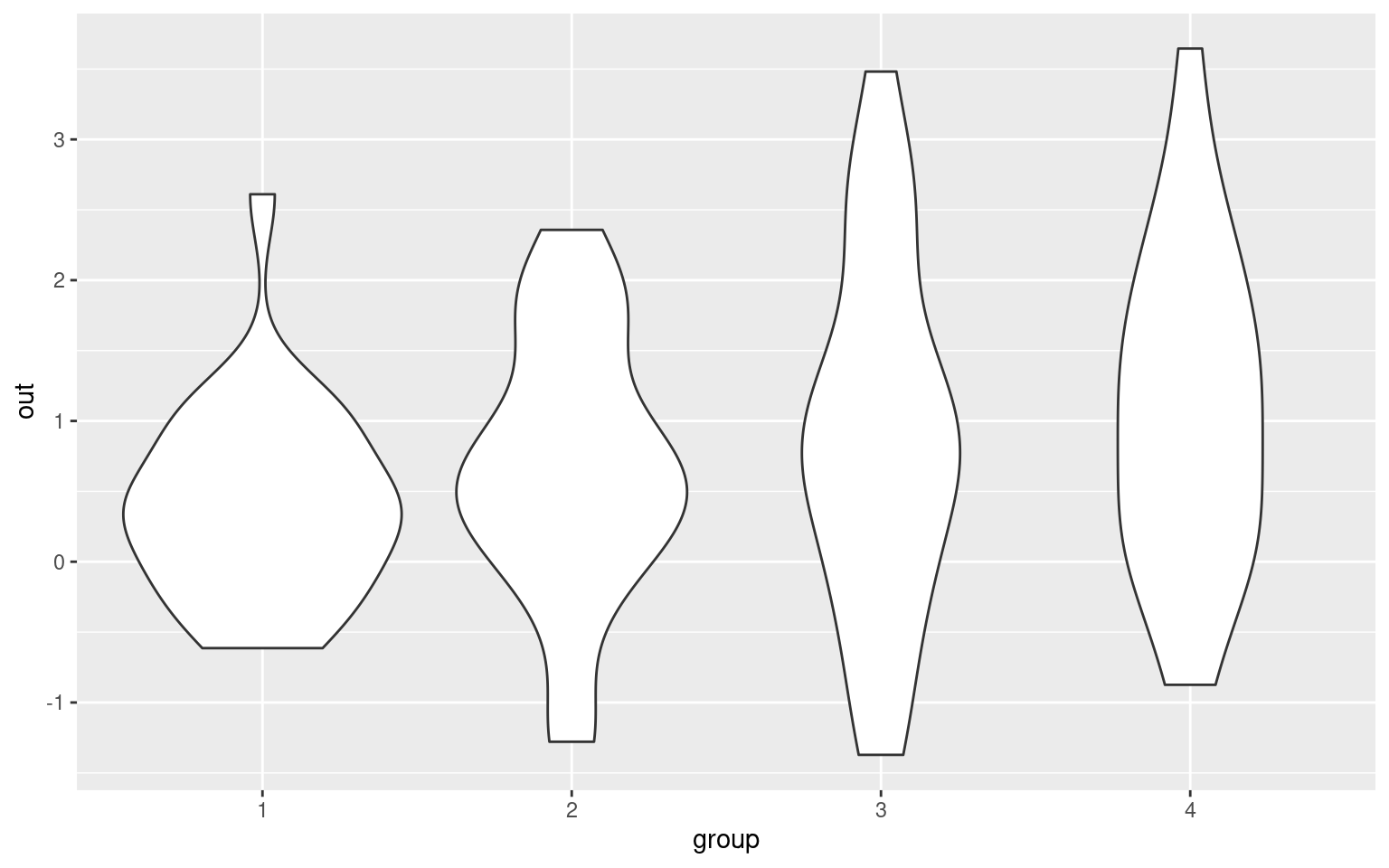
Results are a bit ambiguous–the p-value is 0.13–not really strong evidence for a lack of an effect. To calculate \(f^2\), we could either make an lm or do it by hand:
r2 <- cor(out, model$fit)^2
print(r2)
[1] 0.05683526f2 <- r2/(1 - r2)
f2[1] 0.06026016Now, f2 is .06. How many participants would we have to have run to find a significant effect?
pwr.f2.test(u = 3, f2 = 0.0603, sig.level = 0.05, power = 0.8)
     Multiple regression power calculation

              u = 3
              v = 180.7598
             f2 = 0.0603
      sig.level = 0.05
          power = 0.8
v=180–almost twice as many!
Power for Chi-squared (\(\chi^2\) ) tests
Chi-squared test of ‘goodness of fit’.
Normally, we use a \(\chi^2\) test to compare two sets of proportions. The effect size it uses is w, which can be computed using the ES.w1 function. Suppose we observed a set of rolls of dice (300 rolls), and we suspect that the die may be biased. How many times would we have to roll it to be confident it was fair?
table <- cbind(c(0.1652, 0.1302, 0.1435, 0.1702, 0.1853, 0.2053), rep(1, 6)/6)

ES.w1(table[, 1], table[, 2])
[1] 0.1522623The effect size is about .15. Notice that in the example above, we
are comparing a fair die to one that is unfair. Since each element of
the table represents a different outcome, we are testing whether the one
distribution matches the null (equal-probability) distribution and we
use ES.w1.
test <- pwr.chisq.test(w = 0.15, df = 5, sig.level = 0.05, power = 0.8)
test
     Chi squared power calculation

              w = 0.15
              N = 570.1158
             df = 5
      sig.level = 0.05
          power = 0.8

NOTE: N is the number of observationsplot(test)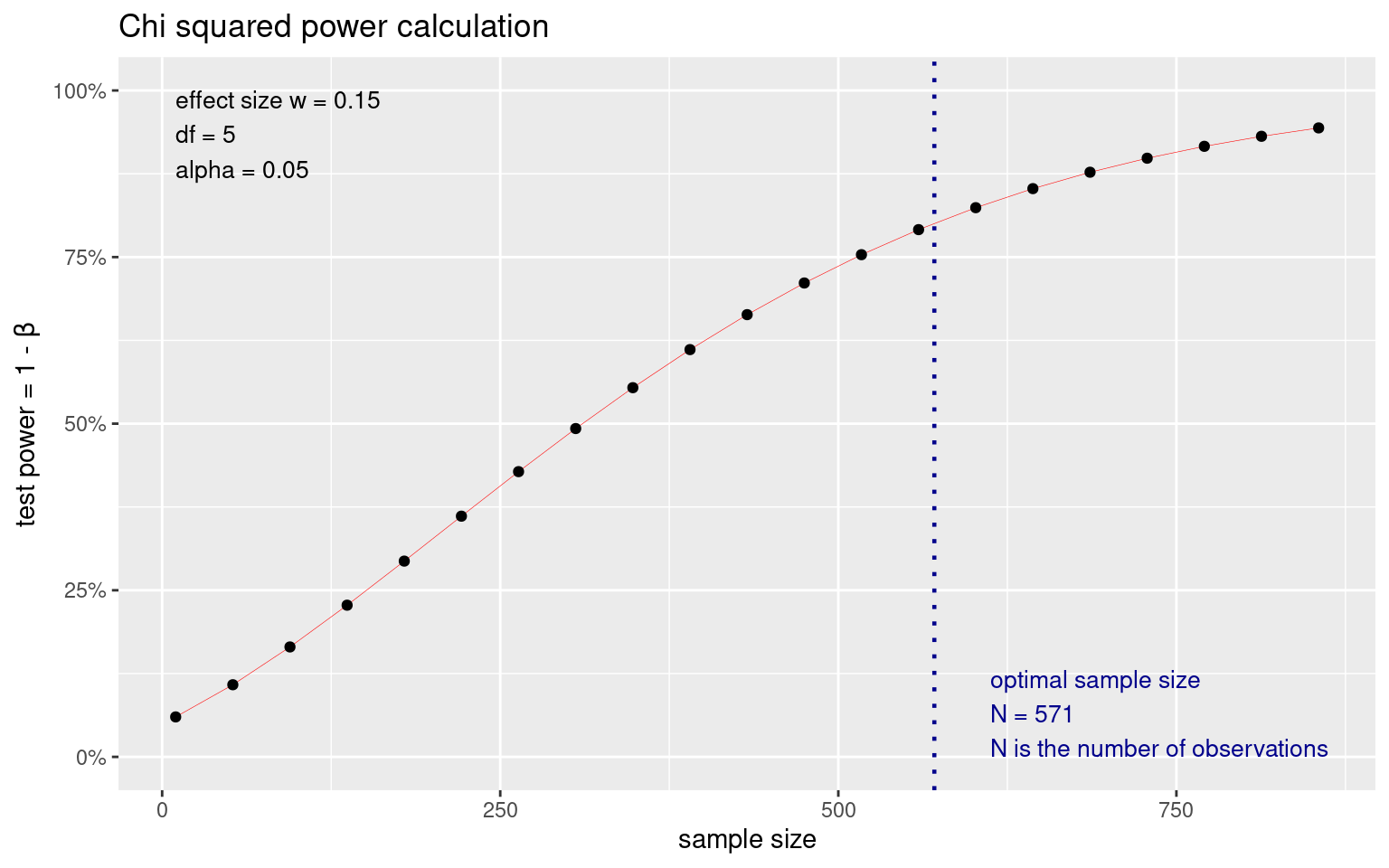
This suggests that for a die with a bias that we observed, we’d need N=571+ to detect the bias 80% of the time, and probably around 1000 rolls to detect it 95% of the time. This might be worthwhile if you were a casino trying to ensure there is no small bias in the dice you purchase that could be used by a player to gain an advantage against the house.
Chi-squared test of association
The other effect size calculation ES.w2 is useful in
slightly different situations. Don’t get the two confused because they
produce different values. ES.w1 assumes that the null hypothesis is the
first argument (i.e., equal probability), whereas ES.w2 assumes that the
null is the model that would be produced if the rows and column margins
were independent. In the example vignette, the demonstration for ES.w2
does not really make any sense, but the effect size for ES.w2 is
comparing the observed vs the independent outcome, whereas ES.w1 is just
comparing the second distribution to the first.
Direct test of Proportions
If you have accuracy data or some proportion, you might want to do a power test to see how large of a sample you need to find a difference. For example, if you have an accuracy of 75%, compared to one of 80%. You use the pwr.2p.test for this, but need to use ES.h to calculate the effect size h.
es <- ES.h(0.8, 0.75)
es
[1] 0.1199023test <- pwr.2p.test(h = es, sig.level = 0.05, power = 0.8)
test
     Difference of proportion power calculation for binomial distribution (arcsine transformation)

              h = 0.1199023
              n = 1091.896
      sig.level = 0.05
          power = 0.8
    alternative = two.sided

NOTE: same sample sizesplot(test)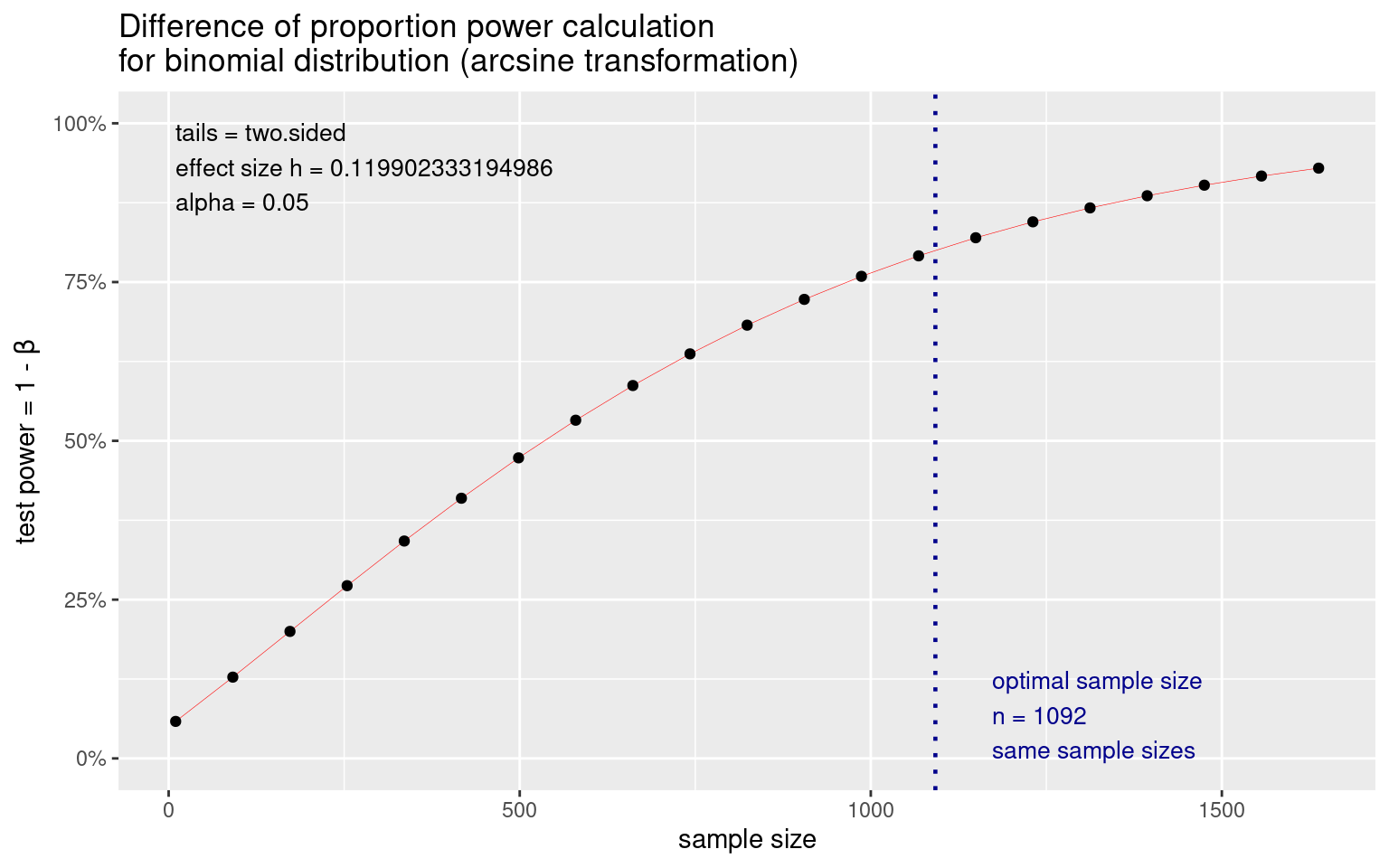
So, 5% difference might require more than 1000 observations per group to be sure to find. Most two-category data sets will obey this principle. This includes tests of whether gender differs by major, conversion rate in A/B testing, etc.
Power for BayesFactor or other tests
The power analysis library really just performs an analytic calculation based on the statistical models being used, but you could estimate the same thing via monte carlo simulation. For complex models, analyses, and the like you may need to do that yourself. I do not know of a power analysis function for bayes factor, but we could simulate it. For example, for our groupA/groupB comparison before, we can see that the full data set produces a large Bayes factor (173) but the small data set produces no substantial difference (.77):
library(BayesFactor)
ttestBF(groupA, groupB)
Bayes factor analysis
--------------
[1] Alt., r=0.707 : 173.0584 ±0%
Against denominator:
Null, mu1-mu2 = 0
---
Bayes factor type: BFindepSample, JZSttestBF(groupA[1:10], groupB[1:10])Bayes factor analysis
--------------
[1] Alt., r=0.707 : 0.7746119 ±0%
Against denominator:
Null, mu1-mu2 = 0
---
Bayes factor type: BFindepSample, JZSLet’s calculate the effect size based on our pilot experiment of 10 participants in each group:
library(effectsize)
cohens_d(groupA[1:10], groupB[1:10])
Cohen's d | 95% CI
-------------------------
-0.62 | [-1.51, 0.28]
- Estimated using pooled SD.cohens_d(groupA, groupB)Cohen's d | 95% CI
--------------------------
-0.56 | [-0.84, -0.27]
- Estimated using pooled SD.This shows d=.62, which is close (but a little larger) than the d for the larger population. We can do some simulations to see the distribution of Bayes Factors for an effect size of .62, across different sample sizes:
samplesizes <- c(10, 25, 50, 100, 150, 200)  ##size of experiments
reps <- 250  ##number of experiments to sample

data <- data.frame(samplesize = rep(samplesizes, each = reps), reps = rep(reps, length(samplesizes)),
    BF = NA)


for (i in 1:nrow(data)) {
    if (i%%100 == 0)
        print(paste(i, "of", reps * length(samplesizes)))
    # sample data points
    g1 <- rnorm(data$samplesize[i], mean = 0, sd = 1)
    g2 <- rnorm(data$samplesize[i], mean = 0.62, sd = 1)
    data$BF[i] <- ttestBF(g1, g2)
}
[1] "100 of 1500"
[1] "200 of 1500"
[1] "300 of 1500"
[1] "400 of 1500"
[1] "500 of 1500"
[1] "600 of 1500"
[1] "700 of 1500"
[1] "800 of 1500"
[1] "900 of 1500"
[1] "1000 of 1500"
[1] "1100 of 1500"
[1] "1200 of 1500"
[1] "1300 of 1500"
[1] "1400 of 1500"
[1] "1500 of 1500"We can look at the distribution of Bayes factors. Suppose we choose a criterion of log(BF)=+3 as the equivalent of power:
library(ggplot2)
ggplot(data, aes(x = as.factor(samplesize), y = log(BF))) + geom_violin(fill = "gold") +
facet_wrap(~reps) + geom_abline(intercept = 3, slope = 0) + theme_minimal()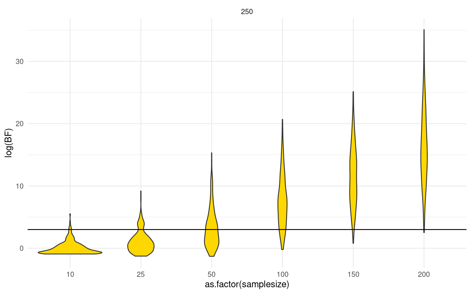 We can examine the probability of finding such a result by counting how
many experiments in each case pass that criterion:
We can examine the probability of finding such a result by counting how
many experiments in each case pass that criterion:
library(tidyverse)
data %>%
    mutate(success = log(BF) > 3) %>%
    group_by(samplesize, reps) %>%
    summarize(meanBF = mean(log(BF)), meanSuccess = mean(success)) %>%
    pivot_longer(cols = meanBF:meanSuccess) %>%
    ggplot(aes(x = samplesize, y = value)) + geom_point() + geom_line() + facet_wrap(~name,
    scales = "free") + theme_bw()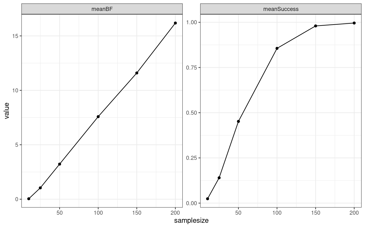
If you did such an analysis, you could report you performed a monte carlo simulation to evaluate the probability that a Bayes Factor t-test produced a value of at least 3.0 using a D=.62, and found that a experiments with 100 in each group produced this effect approximately 80% of the time, and that the mean \(log(BF)\) in for experiments of this size was 7.5.
Other power calculations
the pwr package includes several other power calculation functions that are useful in some particular situations, but we won’t otherwise cover here. The same logic we used for the BayesFactor test could be used for any test that is complicated enough that a pwr function is not available.