Testing and Modeling Multiple Dependent Variables
Suppose you measured two groups or conditions and have a lot of relatively weak measures of difference. You might find that each of the measures are correlated, and measure related constructs. Whether or not the individual measures show significant differences between groups, it might be nice to construct a composite of the DVs. But what is the right way to do that?
There are some problems to think about. Different measures might be negatively correlated with one another, so averaging them would wipe out any effect. Or they may be of different magnitudes (e.g., completion time in seconds for one task, and accuracy for another). If you averaged these, one would swamp the other. Even if you had the same scale (two likert-scale responses), differences in variance could make averaging together problematic.
Keeping them separate is also not always ideal. This produces multiple tests, and so you would have a greater chance of a false alarm. On the other hand, you may have several weak signals–each of which are noisy and none of which are significantly different, even if a composite score might be.
There have been a number of procedures and tests developed to solve this problem. These include:
- Hotellings T2: a generalization of the t-test for multiple DVs
- The MANOVA Procedure: a generalization of ANOVA for multiple DVs
- Canonical Correlation Analysis: correlating two sets of measures
Hotelling T2
The MANOVA is an extension of the ANOVA that attempts to run an ANOVA on a number of dependent measures, combining them optimally.
We will start with an example data set in which three outcome variables are each weakly related to a group membership:
library(Hotelling)
library(ggplot2)
library(ICSNP)
library(reshape2)
set.seed(1000)
n <- 350
group <- rep(1:2, each = n)
xs <- rnorm(n * 2, mean = group * 0.2, sd = 1.4)
ys <- rnorm(n * 2, mean = 4 + group * 1.5, sd = 15)
zs <- rnorm(n * 2, mean = 3 - group * 0.2, sd = 0.9)

ggplot(data.frame(group, xs, ys), aes(x = xs, y = ys, color = group)) + geom_point() +
    labs(title = "X versus Y")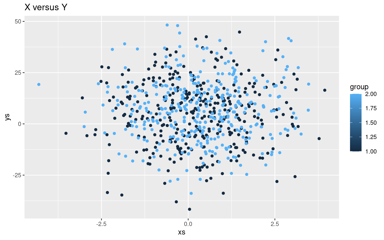
ggplot(data.frame(group, xs, zs), aes(x = xs, y = zs, color = group)) + geom_point() +
    labs(title = "X versus Z")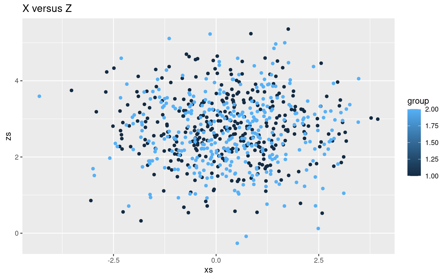
long <- melt(data.frame(group, xs, ys, zs), id.vars = c("group"))
long$group <- as.factor(long$group)
ggplot(data = long, aes(x = (group), y = value)) + geom_violin(aes(fill = group),
    colour = "grey20", scale = "width") + facet_wrap(~variable) + theme_minimal() +
    scale_fill_manual(values = c("gold", "cadetblue3"))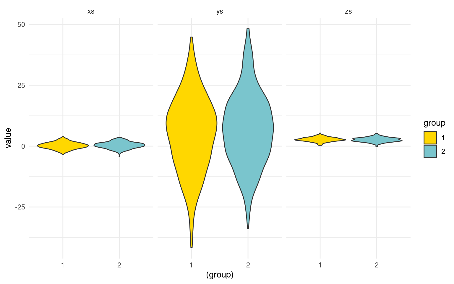
Notice that the three values we measured are on different scales, and they differ in different ways across groups.
t.test(xs ~ group)
    Welch Two Sample t-test

data:  xs by group
t = -1.3874, df = 697.9, p-value = 0.1658
alternative hypothesis: true difference in means between group 1 and group 2 is not equal to 0
95 percent confidence interval:
 -0.33887615  0.05825459
sample estimates:
mean in group 1 mean in group 2
0.2250053 0.3653161 t.test(ys ~ group)
    Welch Two Sample t-test

data:  ys by group
t = -1.7294, df = 696.93, p-value = 0.08419
alternative hypothesis: true difference in means between group 1 and group 2 is not equal to 0
95 percent confidence interval:
 -4.2298935  0.2680513
sample estimates:
mean in group 1 mean in group 2
5.006313 6.987234 t.test(zs ~ group)
    Welch Two Sample t-test

data:  zs by group
t = 1.7669, df = 697.25, p-value = 0.07768
alternative hypothesis: true difference in means between group 1 and group 2 is not equal to 0
95 percent confidence interval:
 -0.01332771  0.25302765
sample estimates:
mean in group 1 mean in group 2
        2.75949         2.63964
None of these three measures differ significantly at a p<.05 level. Furthermore, the values are on different scales, and for some of them group 1 is higher, while for others group 1 is lower. If we had a high ICC, we might consider making a composite score-averaging these together, and trying to look at the measure that way. In this case, this would not be possible unless we either had some theory (expectations about positive/negative difference and scaling), or did some normalization to bring the measures all onto the same scale. So in an ideal world, maybe we would know something about the data and do this:
x2 <- xs/0.2
y2 <- (ys - 4)/1.5
z2 <- -(zs - 3)/(0.2)

tmp <- data.frame(group = as.factor(rep(group, 3)), val = c(x2, y2, z2), xyz = rep(c("X",
    "Y", "Z"), each = n))

ggplot(tmp, aes(x = group, y = val, col = group)) + geom_violin(aes(fill = group),
    colour = "grey20", scale = "width") + geom_jitter(color = "grey30", width = 0.05,
    height = 0) + facet_wrap(~xyz) + theme_minimal() + scale_fill_manual(values = c("gold",
    "cadetblue3"))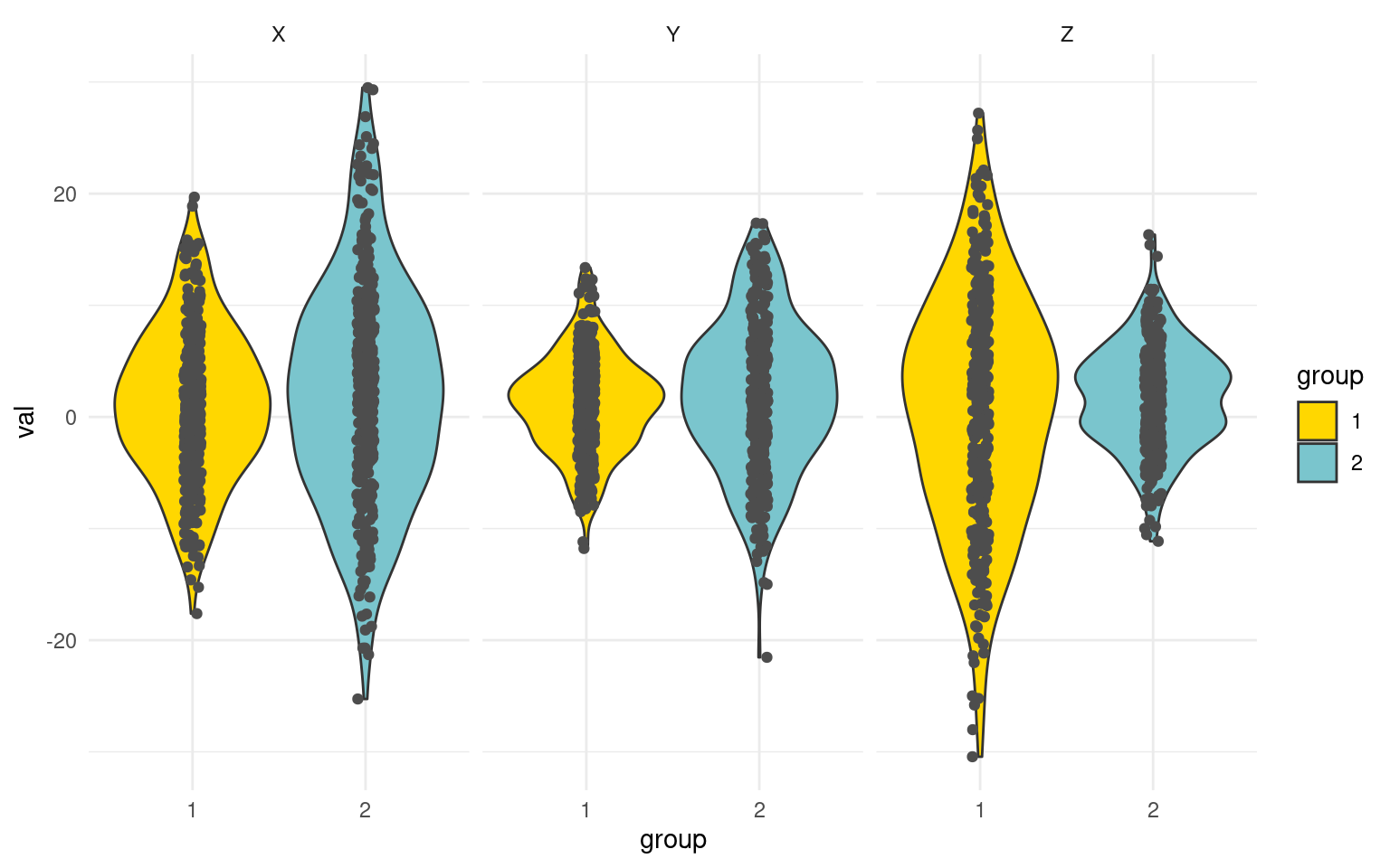
composite <- rowMeans(cbind(x2, y2, z2))
t.test(tmp$val ~ as.factor(tmp$group))
    Welch Two Sample t-test

data:  tmp$val by as.factor(tmp$group)
t = -2.6858, df = 2096.8, p-value = 0.007292
alternative hypothesis: true difference in means between group 1 and group 2 is not equal to 0
95 percent confidence interval:
 -1.511823 -0.235789
sample estimates:
mean in group 1 mean in group 2
      0.9994848       1.8732907
If we get lucky and have a good way of combining multiple values, we can still do a simple t-test. An alternative is the Hotelling \(T^2\) test. This tests whether there is a difference between the groups on the three measures altogether. Hotelling’s \(T^2\) is available from several packages. But the way you call it differs across packages, so you need to be careful:
Hotelling test from ICSNP
HotellingsT2(cbind(xs, ys, zs) ~ group)
    Hotelling's two sample T2-test

data:  cbind(xs, ys, zs) by group
T.2 = 2.7408, df1 = 3, df2 = 696, p-value = 0.04244
alternative hypothesis: true location difference is not equal to c(0,0,0)
hotelling.test from Hotelling package
Previously, the Hotelling package had a function called hotel.test that worked differently from HotellingsT2. In recent versions this has been replaced by hotelling.test, that permits specifying the dependent measures either as a matrix or with \(+\) syntax on the left of the ~ sign:
## From Hotelling package
print(hotelling.test(cbind(xs, ys, zs) ~ group))  ##This won't work in earlier versions of hotel.test.
Test stat: 8.2459
Numerator df: 3
Denominator df: 696
P-value: 0.04244 print(hotelling.test(xs + ys + zs ~ group)) ##correct; value is the same as ICSNPTest stat: 8.2459
Numerator df: 3
Denominator df: 696
P-value: 0.04244 Notice that the sign and scale of the components don’t matter– z is negatively related to the others, but if we reverse code it, the results are the same: ##Negatively code z
z2 <- 5 - zs

print(hotelling.test(xs + ys + z2 ~ group))
Test stat: 8.2459
Numerator df: 3
Denominator df: 696
P-value: 0.04244 print(HotellingsT2(cbind(xs, ys, z2) ~ group))
    Hotelling's two sample T2-test

data:  cbind(xs, ys, z2) by group
T.2 = 2.7408, df1 = 3, df2 = 696, p-value = 0.04244
alternative hypothesis: true location difference is not equal to c(0,0,0)
Similarly, if we reduce scale of one of the components (y), everything stays the same:
y2 <- ys/10

print(hotelling.test(xs + y2 + z2 ~ group))
Test stat: 8.2459
Numerator df: 3
Denominator df: 696
P-value: 0.04244 print(HotellingsT2(cbind(xs, y2, z2) ~ group))
    Hotelling's two sample T2-test

data:  cbind(xs, y2, z2) by group
T.2 = 2.7408, df1 = 3, df2 = 696, p-value = 0.04244
alternative hypothesis: true location difference is not equal to c(0,0,0)
So, Hotelling’s \(T^2\) provides a way of creating sort of a composite score, without worrying about the scale or coding direction of the components. Notice that each individual component did not differ significantly across groups, but the set of three did. This also protects against multiple testing–if we’d measured 10 things and expected them all to differ a little but none did, we’d still have a high chance of a type-II false alarm error. Here, we do just one test. However, notice that the \(T^2\) was not as strong as our “theory-based” composite score above, so we could do better if we have a principled method for combining values (and we were right).
Adding garbage does not help!
xx <- rnorm(700)
yy <- rnorm(700)
print(hotelling.test(xs + y2 + z2 + xx + yy ~ group))
Test stat: 9.3857
Numerator df: 5
Denominator df: 694
P-value: 0.09805 MANOVA: Extending to Multiple Groups
Just as we use one-way and multi-way ANOVA to generalize the t-test, we use the MANOVA (‘multivariate analysis of variance’) to generalize \(T^2\). Sometimes people refer to the Wilks’s Lambda as the alternative to MANOVA corresponding to the one-way ANOVA, but this is mostly nomenclature. R will sometimes do this automatically if given the right inputs. The simplest version is of course the two-group version, and we can see that the car library Anova will produce the same F test as Hotelling. The Manova() function is basically a specialized name for the same analysis.
library(car)
lm(cbind(xs, ys, zs) ~ group)
Call:
lm(formula = cbind(xs, ys, zs) ~ group)

Coefficients:
             xs        ys        zs
(Intercept)   0.08469   3.02539   2.87934
group 0.14031 1.98092 -0.11985anova(lm(cbind(xs, ys, zs) ~ group))Analysis of Variance Table
Df Pillai approx F num Df den Df Pr(>F)
(Intercept) 1 0.90204 2136.32 3 696 < 2e-16 ***
group 1 0.01168 2.74 3 696 0.04244 *
Residuals 698
---
Signif. codes: 0 '***' 0.001 '**' 0.01 '*' 0.05 '.' 0.1 ' ' 1manova(lm(cbind(xs, ys, zs) ~ group))Call:
manova(lm(cbind(xs, ys, zs) ~ group))
Terms:
group Residuals
xs 3.45 1249.39
ys 686.71 160271.31
zs 2.51 562.02
Deg. of Freedom 1 698
Residual standard errors: 1.337891 15.15305 0.8973211
Estimated effects may be unbalancedAnova(lm(cbind(xs, ys, zs) ~ group))
Type II MANOVA Tests: Pillai test statistic
      Df test stat approx F num Df den Df  Pr(>F)
group  1  0.011676   2.7408      3    696 0.04244 *
---
Signif. codes: 0 '***' 0.001 '**' 0.01 '*' 0.05 '.' 0.1 ' ' 1Manova(lm(cbind(xs, y2, z2) ~ group))
Type II MANOVA Tests: Pillai test statistic
      Df test stat approx F num Df den Df  Pr(>F)
group  1  0.011676   2.7408      3    696 0.04244 *
---
Signif. codes:  0 '***' 0.001 '**' 0.01 '*' 0.05 '.' 0.1 ' ' 1
Again, it doesn’t matter the scale or direction of the individual DVs.
what happens when we have three groups? We can actually give a multiple-column dependent measure to lm, but it does not really do what we might expect:
set.seed(1001)
val <- rnorm(500)
group <- as.factor(sample(c("A", "B", "C"), 500, replace = T))
out1 <- 30 + val * 0.3 - as.numeric(group) * 0.25 + rnorm(500) * 4
out2 <- 40 - val * 0.4 + as.numeric(group) * 0.3 + rnorm(500) * 4

dat1 <- data.frame(val, group, out1, out2)
dat2 <- data.frame(val, group, out = c(out1, out2), measure = rep(c("out1", "out2"),
    each = 500))


ggplot(dat2, aes(x = val, y = out, color = group)) + geom_point() + facet_wrap(~measure)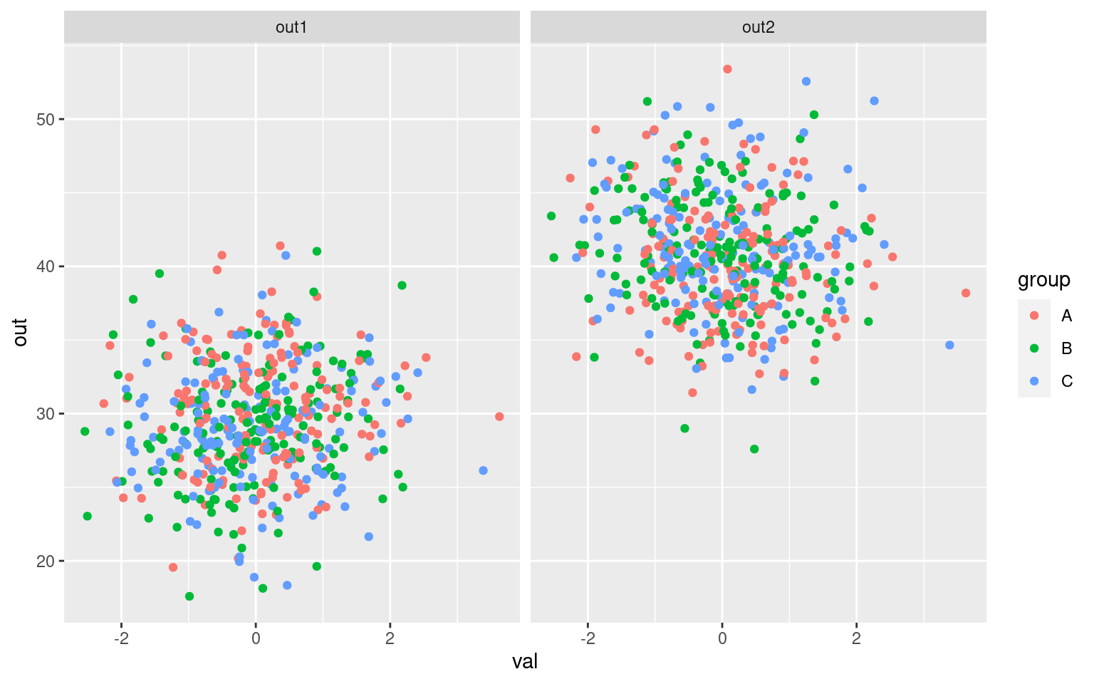
## this just does things 'in parallel'
lm1 <- lm(cbind(out1, out2) ~ val + group)
summary(lm1)
Response out1 :
Call:
lm(formula = out1 ~ val + group)
Residuals:
Min 1Q Median 3Q Max
-11.1879 -2.5912 -0.0488 2.5191 11.6169
Coefficients:
Estimate Std. Error t value Pr(>|t|)
(Intercept) 30.2884 0.3088 98.071 < 2e-16 ***
val 0.3327 0.1785 1.864 0.06295 .
groupB -1.1809 0.4323 -2.732 0.00653 **
groupC -1.2174 0.4342 -2.804 0.00524 **
---
Signif. codes: 0 '***' 0.001 '**' 0.01 '*' 0.05 '.' 0.1 ' ' 1
Residual standard error: 3.941 on 496 degrees of freedom
Multiple R-squared: 0.02762, Adjusted R-squared: 0.02173
F-statistic: 4.695 on 3 and 496 DF, p-value: 0.003039
Response out2 :
Call:
lm(formula = out2 ~ val + group)
Residuals:
Min 1Q Median 3Q Max
-13.0958 -2.7026 -0.2365 2.5003 13.2246
Coefficients:
Estimate Std. Error t value Pr(>|t|)
(Intercept) 40.2092 0.3084 130.392 < 2e-16 ***
val -0.4676 0.1782 -2.623 0.00897 **
groupB 0.7005 0.4316 1.623 0.10523
groupC 1.1582 0.4335 2.672 0.00779 **
---
Signif. codes: 0 '***' 0.001 '**' 0.01 '*' 0.05 '.' 0.1 ' ' 1
Residual standard error: 3.935 on 496 degrees of freedom
Multiple R-squared: 0.02858, Adjusted R-squared: 0.0227
F-statistic: 4.864 on 3 and 496 DF, p-value: 0.002414Here, it really just runs a regression twice, once on each outcome variable. But if we give this lm to anova, it will do a MANOVA
library(car)
anova(lm1)
Analysis of Variance Table
Df Pillai approx F num Df den Df Pr(>F)
(Intercept) 1 0.99363 38603 2 495 < 2.2e-16 ***
val 1 0.02359 6 2 495 0.002715 **
group 2 0.03591 5 4 992 0.001239 **
Residuals 496
---
Signif. codes: 0 '***' 0.001 '**' 0.01 '*' 0.05 '.' 0.1 ' ' 1However, this uses a “Type-I” MANOVA. Because we have multiple predictors, maybe we want a type-II MANOVA, which car::Anova and car::Manova do.
## these two produce the same results:
Anova(lm1)
Type II MANOVA Tests: Pillai test statistic
      Df test stat approx F num Df den Df   Pr(>F)
val    1  0.021684   5.4857      2    495 0.004402 **
group  2  0.035909   4.5342      4    992 0.001239 **
---
Signif. codes: 0 '***' 0.001 '**' 0.01 '*' 0.05 '.' 0.1 ' ' 1Manova(lm1)
Type II MANOVA Tests: Pillai test statistic
      Df test stat approx F num Df den Df   Pr(>F)
val    1  0.021684   5.4857      2    495 0.004402 **
group  2  0.035909   4.5342      4    992 0.001239 **
---
Signif. codes:  0 '***' 0.001 '**' 0.01 '*' 0.05 '.' 0.1 ' ' 1
Interpreting the MANOVA Statistics
When computing a standard ANOVA, we are dividing up our variance into pools accounted for by different predictors and combinations of predictors. In MANOVA, instead of variance, we have a covariance matrix that we are trying to do the same thing with. For \(N\) outcomes, this involves \(N\) variance terms, plus \(N*(N-1)/2\) covariance (correlation) terms. The test statistics work by computing eigenvalues of this covariance matrix, and denote \(\lambda_i\) as the \(ith\) eigenvalue. Most test statistics are function of these \(\lambda\) values, and there are a number of ways to combine these, and each has its own null-hypothesis distribution that is generally related to the F test.
The following is from: https://en.wikiversity.org/wiki/Advanced_ANOVA/MANOVA
Choose from among these multivariate test statistics to assess whether there are statistically significant differences across the levels of the IV(s) for a linear combination of DVs. In general Wilks’ \(\lambda\) is recommended unless there are problems with small N, unequal ns, violations of assumptions, etc. in which case Pillai’s trace is more robust:
Roy’s greatest characteristic root
- Tests for differences on only the first discriminant function
- Most appropriate when DVs are strongly interrelated on a single dimension
- Highly sensitive to violation of assumptions - most powerful when all assumptions are met
Wilks’ lambda (\(\Lambda\))
- Most commonly used statistic for overall significance
- Considers differences over all the characteristic roots
- The smaller the value of Wilks’ lambda, the larger the between-groups dispersion
Hotelling’s trace
- Considers differences over all the characteristic roots
Pillai’s criterion
- Considers differences over all the characteristic roots
- More robust than Wilks’; should be used when sample size decreases, unequal cell sizes or homogeneity of covariances is violated
Typically, packages will report Pillai’s criterion or Pillai’s trace. It is the sum of \((\lambda)/(1-\lambda)\), which should remind you of the effect size \(f^2\) used in calculating power, since the eigenvalue is a measure of the proportion of variance. Hotelling’s Trace (or Hotelling-Lawley’s Trace) is the sum of the eigenvalues; Wilks \(\lambda\) is the sum of \(1/(1+\lambda_i)\). Roy’s greatest root is the largest \(\lambda\); essentially considering just the first principle component.
Each of these tests are available for specifying in Anova, but “Pillai” is the default:
Manova(lm1, test.statistic = "Wilks")
Type II MANOVA Tests: Wilks test statistic
      Df test stat approx F num Df den Df   Pr(>F)
val    1   0.97832   5.4857      2    495 0.004402 **
group  2   0.96413   4.5619      4    990 0.001180 **
---
Signif. codes: 0 '***' 0.001 '**' 0.01 '*' 0.05 '.' 0.1 ' ' 1Manova(lm1, test.statistic = "Hotelling-Lawley")
Type II MANOVA Tests: Hotelling-Lawley test statistic
      Df test stat approx F num Df den Df   Pr(>F)
val    1  0.022164   5.4857      2    495 0.004402 **
group  2  0.037162   4.5895      4    988 0.001124 **
---
Signif. codes: 0 '***' 0.001 '**' 0.01 '*' 0.05 '.' 0.1 ' ' 1Manova(lm1, test.statistic = "Roy")
Type II MANOVA Tests: Roy test statistic
      Df test stat approx F num Df den Df    Pr(>F)
val    1  0.022164   5.4857      2    495 0.0044017 **
group  2  0.036008   8.9300      2    496 0.0001549 ***
---
Signif. codes:  0 '***' 0.001 '**' 0.01 '*' 0.05 '.' 0.1 ' ' 1
The different statistics give different interpretations. Roy’s greatest root essentially asks whether there is a difference on the primary dimension of shared variance of the dependent variables. The others consider all the dimensions of shared variance, but combine these differently.
Ultimately, the MANOVA often hides more than it reveals. Many statisticians have recommended you avoid using it unless you really need to, but it can come in handy, and understanding is important for evaluating other research.
Conceptual relationship to PCA
Conceptually, MANOVA is sort of like doing something like the following, which performs a regression on dimensions of a principal components analysis. If you are trying to do something like this, it would usually be better to use the MANOVA directly rather than trying to figure out something ad hoc like predicting eigen vectors ‘by hand’:
E <- eigen(cor((dat1[, 3:4])))
print(E)
eigen() decomposition
$values
[1] 1.0331709 0.9668291
$vectors
[,1] [,2]
[1,] 0.7071068 -0.7071068
[2,] 0.7071068 0.7071068p1 <- as.matrix(dat1[, 3:4]) %*% as.matrix(E$vectors[, 1])
p2 <- as.matrix(dat1[, 3:4]) %*% as.matrix(E$vectors[, 2])
m1 <- (lm(p1 ~ val + group))
summary(m1)
Call:
lm(formula = p1 ~ val + group)

Residuals:
     Min       1Q   Median       3Q      Max
-13.5333  -2.4216  -0.1097   2.7163  11.3580

Coefficients:
            Estimate Std. Error t value Pr(>|t|)
(Intercept) 49.84928    0.31788 156.818   <2e-16 ***
val         -0.09538    0.18372  -0.519    0.604
groupB      -0.33967    0.44495  -0.763    0.446
groupC      -0.04186    0.44686  -0.094    0.925
---
Signif. codes:  0 '***' 0.001 '**' 0.01 '*' 0.05 '.' 0.1 ' ' 1

Residual standard error: 4.057 on 496 degrees of freedom
Multiple R-squared:  0.001911,  Adjusted R-squared:  -0.004126
F-statistic: 0.3165 on 3 and 496 DF, p-value: 0.8134Anova(m1)Anova Table (Type II tests)
Response: p1
Sum Sq Df F value Pr(>F)
val 4.4 1 0.2695 0.6039
group 11.5 2 0.3500 0.7049
Residuals 8162.5 496 m2 <- lm(p2 ~ val + group)
summary(m2)
Call:
lm(formula = p2 ~ val + group)

Residuals:
     Min       1Q   Median       3Q      Max
-10.4104  -2.4849  -0.2255   2.5036  13.4315

Coefficients:
            Estimate Std. Error t value Pr(>|t|)
(Intercept)   7.0150     0.2990  23.458  < 2e-16 ***
val          -0.5658     0.1728  -3.274  0.00113 **
groupB        1.3304     0.4186   3.178  0.00157 **
groupC        1.6798     0.4204   3.996 7.42e-05 ***
---
Signif. codes:  0 '***' 0.001 '**' 0.01 '*' 0.05 '.' 0.1 ' ' 1

Residual standard error: 3.816 on 496 degrees of freedom
Multiple R-squared:  0.05608,   Adjusted R-squared:  0.05037
F-statistic: 9.822 on 3 and 496 DF, p-value: 2.649e-06Anova(m2)Anova Table (Type II tests)
Response: p2
Sum Sq Df F value Pr(>F)
val 156.1 1 10.7188 0.0011346 **
group 258.3 2 8.8685 0.0001643 ***
Residuals 7223.8 496
---
Signif. codes: 0 '***' 0.001 '**' 0.01 '*' 0.05 '.' 0.1 ' ' 1Notice that for two groups, the eigenvectors are essentially the mean and the difference between the observations. As the number of outcomes increases, these would be less constrained. If you look at the F tests for each predictor, you will see that the values are very similar to those produced in the PCA version (either on average, or max values, etc.). But this means that, depending on the test statistic, a MANOVA might also be considering strange and non-intuitive combinations of variables. Importantly, the group of dependent measures do not need to be correlated. Consider the following dependent variables. Here, out1 and out2 are independent, but group is related to the difference between them. Group is thus also indirectly related to each one, because the difference is larger when one is large or when the other is small (or both). Group2 and out3 are unrelated to the others.
Some statisticians have explored procedures like this for doing ANOVA on PCA (e.g., https://iopscience.iop.org/article/10.1088/1742-6596/1899/1/012103/pdf). According to Abapihi et al. (2021), practitioners sometimes have found the MANOVA difficult to apply because of its strict assumptions, and propose ANOVA on the first principal component as an alternative. It seems like this would be successful if your first dimension is highly interpretable, but I wouldn’t recommend it unless you take the PCA seriously first. For example, if your first component is highly interpretable and accounts for a substantial amount of variance, this might be easily justified, but it is mostly a similar procedure as Roy’s GCR statistic. Other MANOVA statistics will incorporate all dimensions.
set.seed(150)
yout1 <- rnorm(150)
yout2 <- rnorm(150)
yout3 <- rnorm(150)
delta <- ((yout1 - mean(yout1)) - (yout2 - mean(yout2))) + rnorm(150) * 5
group1 <- floor(rank(delta)/50) + 1
group2 <- sample(1:5, replace = T, size = 150)
out <- cbind(yout1, yout2, yout3)
summary(lm(out ~ group1))
Response yout1 :
Call:
lm(formula = yout1 ~ group1)
Residuals:
Min 1Q Median 3Q Max
-2.41516 -0.71119 0.00642 0.75209 2.45372
Coefficients:
Estimate Std. Error t value Pr(>|t|)
(Intercept) -0.21468 0.21687 -0.99 0.324
group1 0.14901 0.09933 1.50 0.136
Residual standard error: 1.008 on 148 degrees of freedom
Multiple R-squared: 0.01498, Adjusted R-squared: 0.008322
F-statistic: 2.25 on 1 and 148 DF, p-value: 0.1357
Response yout2 :
Call:
lm(formula = yout2 ~ group1)
Residuals:
Min 1Q Median 3Q Max
-2.80585 -0.52989 -0.04297 0.60846 2.24696
Coefficients:
Estimate Std. Error t value Pr(>|t|)
(Intercept) 0.40930 0.20202 2.026 0.0446 *
group1 -0.23560 0.09253 -2.546 0.0119 *
---
Signif. codes: 0 '***' 0.001 '**' 0.01 '*' 0.05 '.' 0.1 ' ' 1
Residual standard error: 0.9388 on 148 degrees of freedom
Multiple R-squared: 0.04197, Adjusted R-squared: 0.0355
F-statistic: 6.484 on 1 and 148 DF, p-value: 0.01191
Response yout3 :
Call:
lm(formula = yout3 ~ group1)
Residuals:
Min 1Q Median 3Q Max
-2.99510 -0.70386 -0.03446 0.70520 2.32555
Coefficients:
Estimate Std. Error t value Pr(>|t|)
(Intercept) 0.05673 0.21535 0.263 0.793
group1 -0.03119 0.09864 -0.316 0.752
Residual standard error: 1.001 on 148 degrees of freedom
Multiple R-squared: 0.0006752, Adjusted R-squared: -0.006077
F-statistic: 0.09999 on 1 and 148 DF, p-value: 0.7523Manova(lm(out ~ group1 + group2), test.statistic = "Roy")
Type II MANOVA Tests: Roy test statistic
       Df test stat approx F num Df den Df  Pr(>F)
group1  1  0.053897  2.60501      3    145 0.05412 .
group2  1  0.016187  0.78238      3    145 0.50559
---
Signif. codes: 0 '***' 0.001 '**' 0.01 '*' 0.05 '.' 0.1 ' ' 1Manova(lm(out ~ group1 + group2), test.statistic = "Pillai")
Type II MANOVA Tests: Pillai test statistic
       Df test stat approx F num Df den Df  Pr(>F)
group1  1  0.051140  2.60501      3    145 0.05412 .
group2  1  0.015929  0.78238      3    145 0.50559
---
Signif. codes: 0 '***' 0.001 '**' 0.01 '*' 0.05 '.' 0.1 ' ' 1Manova(lm(out ~ group1 + group2), test.statistic = "Wilks")
Type II MANOVA Tests: Wilks test statistic
       Df test stat approx F num Df den Df  Pr(>F)
group1  1   0.94886  2.60501      3    145 0.05412 .
group2  1   0.98407  0.78238      3    145 0.50559
---
Signif. codes:  0 '***' 0.001 '**' 0.01 '*' 0.05 '.' 0.1 ' ' 1
Relation to Repeated Measures ANOVA
This all seems like it is a bit like a repeated-measures ANOVA. By putting the data in ‘long’ format, we can just combine out1 and out2 into a single DV, then predict the mean difference between the two with a categorical value:
dat2 <- data.frame(val, group, out = c(out1, out2), measure = rep(c("out1", "out2"),
    500))


model.rm <- lm(out ~ val + group + measure, data = dat2)
summary(model.rm)
Call:
lm(formula = out ~ val + group + measure, data = dat2)

Residuals:
     Min       1Q   Median       3Q      Max
-17.3432  -5.8142   0.1021   5.6072  18.0186

Coefficients:
            Estimate Std. Error t value Pr(>|t|)
(Intercept) 35.38334    0.44659  79.231   <2e-16 ***
val         -0.06344    0.22260  -0.285    0.776
groupB      -0.25003    0.53912  -0.464    0.643
groupC      -0.03096    0.54119  -0.057    0.954
measureout2 -0.26154    0.43988  -0.595    0.552
---
Signif. codes:  0 '***' 0.001 '**' 0.01 '*' 0.05 '.' 0.1 ' ' 1

Residual standard error: 6.948 on 995 degrees of freedom
Multiple R-squared:  0.0006802, Adjusted R-squared:  -0.003337
F-statistic: 0.1693 on 4 and 995 DF,  p-value: 0.9541
This might be OK is some situations. But this is assuming that the two measures differ just by a constant. What if they have different scales, different variances, different directional relationships? Just like the t-test above, if we had a theory that could be used to combine these, it might be a better approach, but in this case, we are restricted in the inferences we can make. Notice that for each sub-model, the effects are in different directions, and so cancel out one another if we do it this way. We could sort of do this by predicting all the interactions too, but this begins to get very complicated such that a MANOVA might be preferred.
Relationship to Logistic Regression, PCA, LDA, and Classification
As we can see, although MANOVA seems like it is just a simple extension of ANOVA, it relates to many multi-variate concepts. For Hotelling’s \(T^2\) version, we are attempting to find whether there is a difference between two groups on multiple measures. We could easily turn this around; predicting group membership based on those multiple `predictors’. This is what methods such as logistic regression and linear discriminant analysis do. As we extend to multiple categories in MANOVA, this becomes similar to what some machine classification schemes permit–classifying categories based on multiple observed ‘features’. Finally, we can understand MANOVA as sort of doing regressions on each principle component, and determining a reasonable means of combining those regressions at the end of the day.
Exercise:
The bfi data set in psych has data from a big-five inventory, and includes gender and age. Look at conscientiousness as a subscale, and examine whether it appears to be a coherent factor. Then, use MANOVA to predict the set of conscientiousness questions using gender and age. Does the personality depend on these? Recode age to a categorical 2- or 3-group factor, and test the interaction between gender and age.
library(psych)
library(car)
data(bfi)

dplyr::select(bfi, A1:O5)
A1 A2 A3 A4 A5 C1 C2 C3 C4 C5 E1 E2 E3 E4 E5 N1 N2 N3 N4 N5 O1 O2 O3 O4
61617 2 4 3 4 4 2 3 3 4 4 3 3 3 4 4 3 4 2 2 3 3 6 3 4
61618 2 4 5 2 5 5 4 4 3 4 1 1 6 4 3 3 3 3 5 5 4 2 4 3
61620 5 4 5 4 4 4 5 4 2 5 2 4 4 4 5 4 5 4 2 3 4 2 5 5
O5
61617 3
61618 3
61620 2
[ reached 'max' / getOption("max.print") -- omitted 2797 rows ]lm1 <- lm(as.matrix(dplyr::select(bfi, A1:O5)) ~ bfi$gender)
Manova(lm1)
Type II MANOVA Tests: Pillai test statistic
           Df test stat approx F num Df den Df    Pr(>F)
bfi$gender  1   0.14813   16.763     25   2410 < 2.2e-16 ***
---
Signif. codes:  0 '***' 0.001 '**' 0.01 '*' 0.05 '.' 0.1 ' ' 1
Canonical Correlation Analysis
MANOVA extends ANOVA/regression and allows multiple predictors and multiple outcome variables. A lesser-known alternative is Canonical Correlation Analysis (CCA), which tries to establish the cross-correlation between two sets of variables, and does so by establishing a dimensionality of the relationship.
This is akin to a PCA, but rather than just finding the dimension of variability that is greatest, it finds the dimension of the covariance between the two variables that is the greatest. So, each set of measures A and B have a mapping onto latent variables (like PCA), which we call X and Y. This mapping is done so that the first dimension of X and the first dimension of Y are as highly correlated as we can get. Then, we find another two orthogonal dimensions, which compose the second set of canonical correlations. This can go on until we have N canonical correlations, where N is the smaller of the two numbers of variables.
Packages and resources
- https://stats.idre.ucla.edu/r/dae/canonical-correlation-analysis/
cancorfunction in stats package- CCA package
- candisc package
library(CCA)
matcor(out, cbind(group1, group2))
$Xcor
yout1 yout2 yout3
yout1 1.00000000 -0.06856134 -0.02984807
yout2 -0.06856134 1.00000000 -0.03009671
yout3 -0.02984807 -0.03009671 1.00000000
$Ycor
group1 group2
group1 1.0000000 0.1070147
group2 0.1070147 1.0000000
$XYcor
yout1 yout2 yout3 group1 group2
yout1 1.00000000 -0.06856134 -0.02984807 0.12238444 -0.03493933
yout2 -0.06856134 1.00000000 -0.03009671 -0.20486423 -0.12148177
yout3 -0.02984807 -0.03009671 1.00000000 -0.02598397 -0.04842062
group1 0.12238444 -0.20486423 -0.02598397 1.00000000 0.10701468
group2 -0.03493933 -0.12148177 -0.04842062 0.10701468 1.00000000img.matcor(matcor(out, cbind(group1, group2)))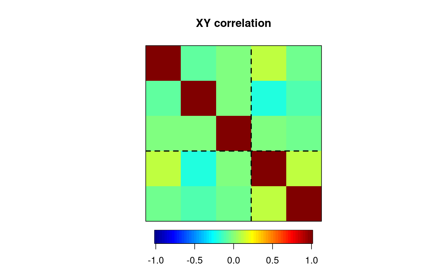
img.matcor(matcor(out, cbind(group1, group2)), type = 2)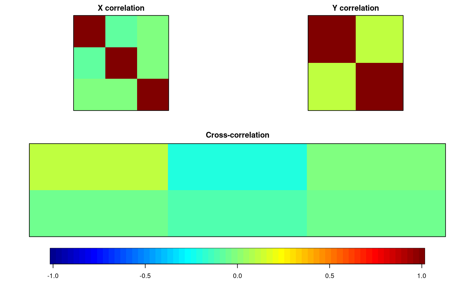
x <- cc(out, cbind(group1, group2))
print(x)
$cor
[1] 0.24555116 0.09975194
$names
$names$Xnames
[1] "yout1" "yout2" "yout3"
$names$Ynames
[1] "group1" "group2"
$names$ind.names
NULL
$xcoef
[,1] [,2]
yout1 -0.3316122 -0.8923137
yout2 0.9470580 -0.3420840
yout3 0.1802280 -0.3832381
$ycoef
[,1] [,2]
group1 -1.0892190 -0.5270819
group2 -0.2316294 0.6476470
$scores
$scores$xscores
[,1] [,2]
[1,] 1.36305021 0.995883466
[2,] -0.56565672 0.507227219
[3,] -0.91210575 1.338943099
[4,] 0.04287964 0.109404897
[5,] -0.40624108 0.911386088
[6,] -0.94537667 0.595946887
[7,] 0.05491903 -0.853656228
[8,] 1.80673300 -0.959494532
[9,] 0.01749876 -0.286410996
[10,] -0.35742517 0.791743077
[11,] 0.50436696 -0.109395258
[12,] 0.45791621 1.929404728
[13,] 1.84623811 -0.978375490
[14,] -0.13690027 1.415658235
[15,] -0.48291423 0.965121629
[16,] -1.56541826 -0.654126001
[17,] 0.12005283 0.220043991
[18,] -0.81618654 -1.359155663
[19,] -1.60095541 0.393913477
[20,] 0.83146701 1.820576387
[21,] 0.92091739 -1.155230595
[22,] -0.68469957 -1.096972683
[23,] -0.25309080 -0.714380944
[24,] 0.57425159 -0.109118293
[25,] -1.05845240 -2.193440426
[26,] 0.19111584 -0.911822474
[27,] 0.03437887 -1.641895806
[28,] 0.20492095 1.615580213
[29,] -0.30816833 -1.963921730
[30,] -0.45679786 0.930771364
[31,] -1.73536337 -0.351629856
[32,] 0.55155071 2.275276390
[33,] -0.41845943 -0.373586254
[34,] -0.10720517 -1.095527309
[35,] -0.55227934 0.573454033
[36,] 1.25759802 -1.056976195
[37,] 0.62647125 -0.771836960
[ reached getOption("max.print") -- omitted 113 rows ]
$scores$yscores
[,1] [,2]
[1,] 1.313293056 -0.02798816
[2,] 1.313293056 -0.02798816
[3,] -0.633515672 -1.72979909
[4,] -1.096774378 -0.43450501
[5,] -1.328403731 0.21314202
[6,] -0.470814043 1.38787100
[7,] -0.633515672 -1.72979909
[8,] -0.239184690 0.74022397
[9,] -0.633515672 -1.72979909
[10,] 1.081663703 0.61965887
[11,] 0.455703369 -1.20271714
[12,] 0.224074016 -0.55507011
[13,] 1.081663703 0.61965887
[14,] 1.544922409 -0.67563520
[15,] 1.081663703 0.61965887
[16,] -0.633515672 -1.72979909
[17,] -1.560033084 0.86078906
[18,] -1.560033084 0.86078906
[19,] -1.328403731 0.21314202
[20,] -0.239184690 0.74022397
[21,] -0.007555337 0.09257693
[22,] -1.096774378 -0.43450501
[23,] 0.850034350 1.26730591
[24,] 0.618404997 1.91495295
[25,] -2.417622771 -0.31393992
[26,] 0.455703369 -1.20271714
[27,] 1.544922409 -0.67563520
[28,] -1.096774378 -0.43450501
[29,] 0.224074016 -0.55507011
[30,] -0.865145025 -1.08215205
[31,] 1.313293056 -0.02798816
[32,] 1.081663703 0.61965887
[33,] -0.470814043 1.38787100
[34,] -1.328403731 0.21314202
[35,] 1.544922409 -0.67563520
[36,] -0.007555337 0.09257693
[37,] -0.007555337 0.09257693
[ reached getOption("max.print") -- omitted 113 rows ]
$scores$corr.X.xscores
[,1] [,2]
yout1 -0.4030366 -0.8692130
yout2 0.9228995 -0.2535793
yout3 0.1625920 -0.3455781
$scores$corr.Y.xscores
[,1] [,2]
group1 -0.2312088 -0.03359224
group2 -0.1069591 0.08979132
$scores$corr.X.yscores
[,1] [,2]
yout1 -0.09896611 -0.08670568
yout2 0.22661905 -0.02529503
yout3 0.03992466 -0.03447209
$scores$corr.Y.yscores
[,1] [,2]
group1 -0.9415913 -0.3367578
group2 -0.4355880 0.9001461plot(x$scores$xscores, x$scores$yscores)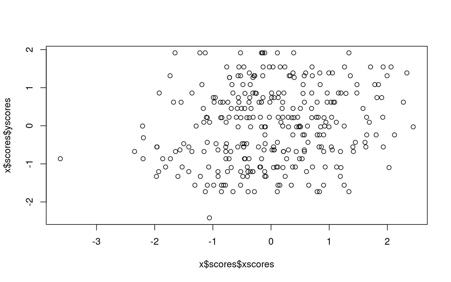
Here, we see the canonical correlation uses two dimensions, because
group only has two variables. The first dimension finds a correlation
between groups of .24, and the second .09.
The first dimension correlates negatively with out1, positively with
out2, and not with out3. The second dimension correlates with out3 only.
On the other side, group 1 and group 2 correlate (negatively) with
dimension 1, and group1 is positively related to dimension 2 but group2
is negatively related to dimension 2.
We can sort of look at what is going on by plotting the first dimension xscores and yscores for each person—this is how each person maps into each of the first canonical correlation dimensions. We can see the correlation is .24, which is a small but probably significant relationship.
cor(x$scores$xscores[, 1], x$scores$yscores[, 1])[1] 0.2455512plot(x$scores$xscores[, 1], x$scores$yscores[, 1])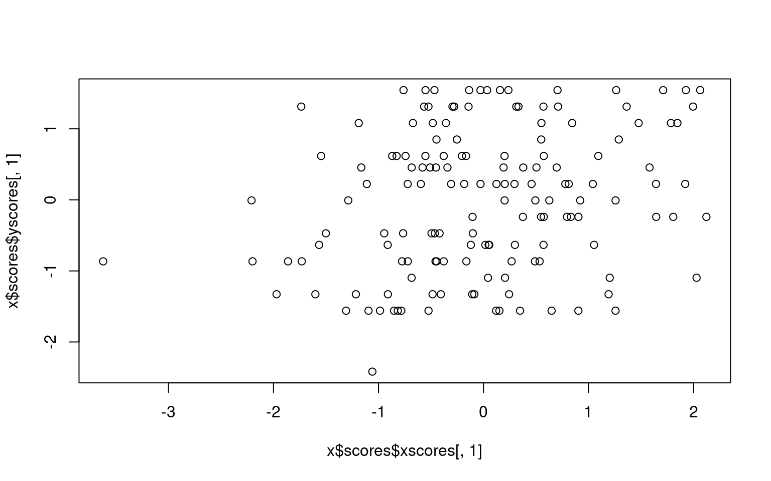
Exercise
Using the psych::BFI data set, use canonical correlation to determine a relationship between agreeableness and conscientiousness. Plot each individual’s scores on the first pair of canonical correlation dimensions against one another.