Beyond Ordinary Least Squares: The Generalized Linear Model (GLM)

Generalized Linear Model (GLM)

The generalized linear model is a framework for fitting and testing versions of the linear regression model that are more flexible than traditional or “ordinary” least squares (OLS). Unlike non-parametric models, GLM models do not “relax” assumptions–they make alternative assumptions, often permitting us to fit different noise distributions, and different non-linear relationships that we might have otherwise used a transformation to achieve.

Some suggested reading/resources include:

R In action, Chapter 13
Faraway’s, “Extending the linear model with R” Chapter 6
Modern Applied Statistics in S, Chapter 7

Assumptions of Ordinary Least Squares (OLS)

Ordinary Least Squares (OLS) regression makes a number of assumptions, which include:

The effects are linear
Error is normally distributed–i.e., the difference between the data and predicted values.
Observations are independent
Variance is uniform across different levels or magnitude of the IVs (no heteroscedascity)
Each observation has equal value in estimating the parameters
(Typically) the best-fitting model is one that minimizes least-squares error

Violations of these assumptions sometimes mean the model is a poor description of the data. At other times, the model will still describe the general pattern of the data accurately, but even if the model is reasonable, violating these will impact our inferential statistics–the extent to which we believe our effects are statistically significant and did not arise from chance. Some of the approaches to this include using transformations to make effects more linear or error more normal. If you have non-independent observations because of repeated measures, you can sometimes use error strata and repeated measures-ANOVA schemes to account for this, or mixed-effects models. But in generally, the fixes to the OLS model get increasingly ad hoc and unprincipled. There are a number of ways that have been used to adopt alternate assumptions and processes we use to extend the model in more systematic ways:

The General Linear Model typically refers to the entire set of linear regression techniques, including the potential for multiple DVS and multiple IVs, including categorical numerical predictors. Thus, ANOVA, MANOVA, regression, t-tests, etc. are all subclasses of this method.
Weighted least-squares, which permit giving different observations different weights.
Maximum likelihood estimation (ML Estimation) is an alternative to least-squares that attempts to find the model parameters that maximize the likelihood of the model. It is especially useful if you have assumed the error is not normal-especially if it is asymmetric. In these cases, least-squares regression will be biased toward the tail of the distribution. Related methods include those that use Bayesian inference, because they also deal with likelihood, but don’t try to maximize it.
Generalized Linear models are extensions to linear regression that incorporate distinct error distributions and transformation functions (called linking functions). These include logistic regression, probit regression, poisson regression, log-linear models, and a handful of similar and related regression methods.
Robust regression methods will attempt to fit models having conditional error distributions that are non-normal, often using alternative means for estimating predictors to avoid biases that might otherwise be introduced.

Maximum Likelihood Estimation

To understand MLE, let’s just remember what likelihood is. Likelihood is calculated for each observed point you are fitting, and it is the height of the error distribution you are fitting. When we fit multiple points, we take the product of all the heights, and try to find a distribution that maximizes this product.

This sometimes leads to nearly identical estimates to the one we get in ordinary least squares. In OLS, we just calculate deviations from the model and try to minimize that, and estimate the error model AFTERWARD. MLE works on the likelihood of the data given the model, and tries to maximize that. Thus, unlike OLS, we need a probability distribution model for this to make sense.

Suppose we observed 100 data points that were taken from a normal distribution. I could make a guess at the distribution (the solid black line below) as a normal distribution with mean =0 and sd = 1. Here, we are just fitting two parameters (mean and sd), but this could be integrated into a regression of arbitrary complexity.

set.seed(111)
data <- rnorm(100)* 1.5+3
hist(data,col="gold",ylim=c(0,50))
mean=0
sd=1
points((-100:100)/10, dnorm((-100:100)/10,mean=mean,sd=sd)*100,type="l",lwd=3)
points(data,  dnorm(data,mean=mean,sd=sd)*100,type="p",cex=1.5)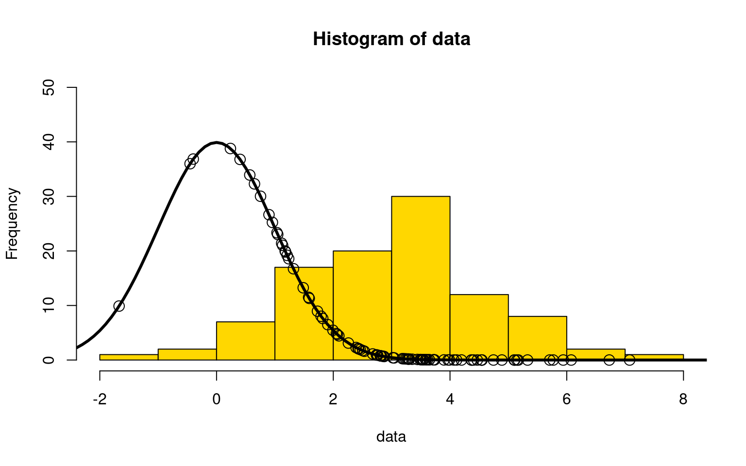

I’ve plotted the distribution we guessed, along with where each point falls on that distribution. Note that the height of the density is scaled to match the histogram, and so they are not really on the same y-axis.

MLE maximizes the product of the likelihood value for each point. If the parameters are \(\mu\) and \(\sigma\), we can represent the likelihood of point \(i\) as \(L(\mu,\sigma)_i\) \(L(\mu,\sigma) = \prod_i { L(\mu,\sigma)_i}\). The values of \(\mu\) and \(\sigma\) that maximize \(L(\mu,\sigma)\) also maximize \(log(L(\mu,\sigma))\), which gives us \(log(L(\mu,\sigma)) =\sum_i{log(L(\mu,\sigma)_i)})\). Numerically, it is a lot easier to add together values, and so we generally use log(likelihood) because it is a faster and more precise calculation. So, calculating the log-likelihood of a model given data is just the sum of the log of the density function–the sum of the log of the curve at each point on the curve.

sum(log(dnorm(data,mean=mean,sd=sd)))

[1] -663.8609

We’d like to find the values of mean and sd that maximize log-like. let’s do a simple grid search:

library(tidyr)
means <- seq(-1,6,.5)
sds <- seq(1,2.5,.25)
loglikes <- matrix(NA, nrow=length(means),ncol=length(sds))
for(i in 1:length(means))
  for(j in 1:length(sds))
  {
    loglikes[i,j] <- sum(log(dnorm(data,mean=means[i],sd=sds[j])))
  }

maxMean <-means[which(rowSums(loglikes==max(loglikes))==1)]
maxSD <- sds[which(colSums(loglikes==max(loglikes))==1)]


data.frame(val=means,loglikes) %>% pivot_longer(cols=2:8) %>%
  mutate(sd=sds[as.numeric(as.factor(name))]) %>%
  mutate(mean=val) %>%
  ggplot(aes(x=mean,y=value,color=sd,group=sd))  + geom_line() +
  theme_bw()  + annotate("text", 1,0,label=paste("Max Mean: ",maxMean)) + 
  annotate("text", 1,-40,label=paste("Max SD: ",maxSD)) + 
  annotate("text",1,-80,label=paste("Max log(Like)= ",round(max(loglikes),2)))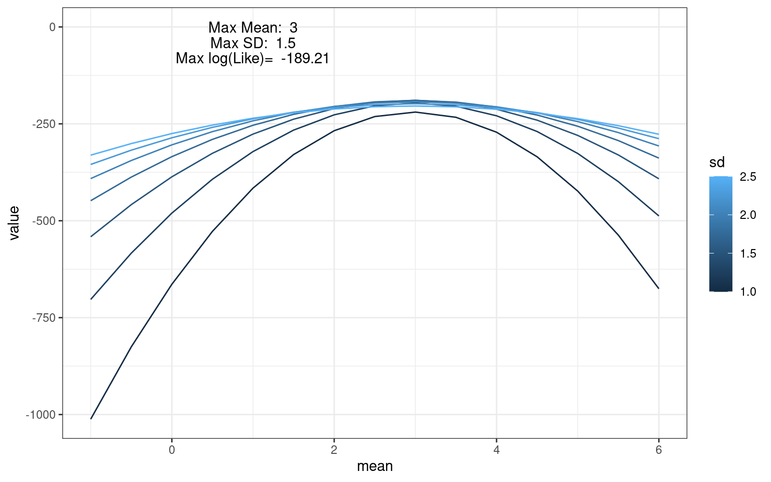

We can easily find that the maximum likelihood combination occurred at mean=3 and sd=1.5, which is close to the values we used to generate the data.

If we happened to get the sd right, we can look at how the log-likelihood is impacted by moving the true mean of the distribution away (from 3 to 2.5 to 2):

par(mfrow=c(1,3))
imean = 1
isd = 6
##the best one
hist(data,col="gold",ylim=c(0,50),main=paste("mean = ",means[imean],", sd =",sds[isd], "\nlog-like=",round(loglikes[imean,isd],2)))
points((-100:100)/10, dnorm((-100:100)/10,mean=means[imean],sd=sds[isd])*100,type="l",lwd=3)
points(data,  dnorm(data,mean=means[imean],sd=sds[isd])*100,type="p",cex=1.5)

imean = 9
isd = 6
##the best one
hist(data,col="gold",ylim=c(0,50),main=paste("mean = ",means[imean],", sd =",sds[isd], "\nlog-like=",round(loglikes[imean,isd],2)))
points((-100:100)/10, dnorm((-100:100)/10,mean=means[imean],sd=sds[isd])*100,type="l",lwd=3)
points(data,  dnorm(data,mean=means[imean],sd=sds[isd])*100,type="p",cex=1.5)


imean = 13
isd = 6
##the best one
hist(data,col="gold",ylim=c(0,50),main=paste("mean = ",means[imean],", sd =",sds[isd], "\nlog-like=",round(loglikes[imean,isd],2)))
points((-100:100)/10, dnorm((-100:100)/10,mean=means[imean],sd=sds[isd])*100,type="l",lwd=3)
points(data,  dnorm(data,mean=means[imean],sd=sds[isd])*100,type="p",cex=1.5)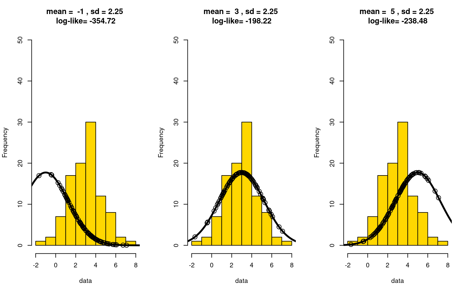

As the mean gets further and further off, the likelihood goes down. Notice that when we get the mean right, more of the points fall at the peak of the distribution. Similarly, suppose we got the mean right, but are searching for the right sd:

par(mfrow=c(1,3))

imean = 9
isd = 1

##the best one
hist(data,col="gold",ylim=c(0,50),main=paste("mean = ",means[imean],", sd =",sds[isd], "\nlog-like=",round(loglikes[imean,isd],2)))
points((-100:100)/10, dnorm((-100:100)/10,mean=means[imean],sd=sds[isd])*100,type="l",lwd=3)
points(data,  dnorm(data,mean=means[imean],sd=sds[isd])*100,type="p",cex=1.5)


imean = 9
isd = 3

##the best one
hist(data,col="gold",ylim=c(0,50),main=paste("mean = ",means[imean],", sd =",sds[isd], "\nlog-like=",round(loglikes[imean,isd],2)))
points((-100:100)/10, dnorm((-100:100)/10,mean=means[imean],sd=sds[isd])*100,type="l",lwd=3)
points(data,  dnorm(data,mean=means[imean],sd=sds[isd])*100,type="p",cex=1.5)


imean = 9
isd = 7

##the best one
hist(data,col="gold",ylim=c(0,50),main=paste("mean = ",means[imean],", sd =",sds[isd], "\nlog-like=",round(loglikes[imean,isd],2)))
points((-100:100)/10, dnorm((-100:100)/10,mean=means[imean],sd=sds[isd])*100,type="l",lwd=3)
points(data,  dnorm(data,mean=means[imean],sd=sds[isd])*100,type="p",cex=1.5)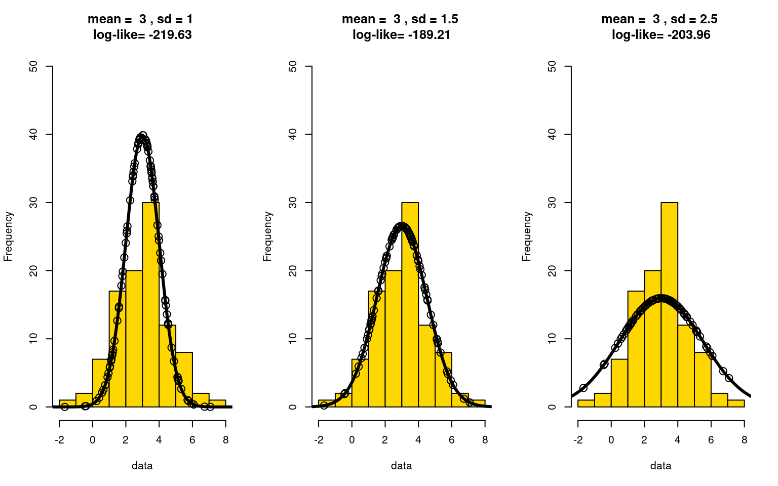

Notice that now, when we under-estimate the standard deviation (left), the likelihood values near the peak give greater values, but we underestimate those in the tails. This can be very costly, because those values are near 0 and have a huge impact on the log-likelihood. On the other hand, if we over-estimate the sd, the peak gets counted less–and this is where most of the points are. The MLE is the point at which these balance out perfectly, which is close to what we see in the center.

Note that the maximum likelihood finds a particular combination of parameters that maximize the likelihood. But as we saw in the likelihood graphs, there are large areas of parameters that are almost as likely, and could easily have generated the data we saw. Another approach is to identify the distribution of the parameters that could have generated the data—this is done with a Bayesian estimation approach, and the distributions are called posterior estimates (the distribution of values given data).

So, with MLE, we fit the entire distribution to the data. That means that if we have a data distribution that is not normal, we could fit a non-normal distribution. Consider this skewed data, which we can fit with a weibull distribution, which has two parameters; scale and shape. we will start with a simple weibull distribution just to show basically how it looks.

set.seed(101)
a <- exp(1.3+.9*rnorm(50))
hist(a,breaks=0:20,ylim=c(0,15),col="gold")
points(0:200/10,dweibull(0:200/10,.2,.3)*50,type="l")
points(a,dweibull(a,.2,.3)*50)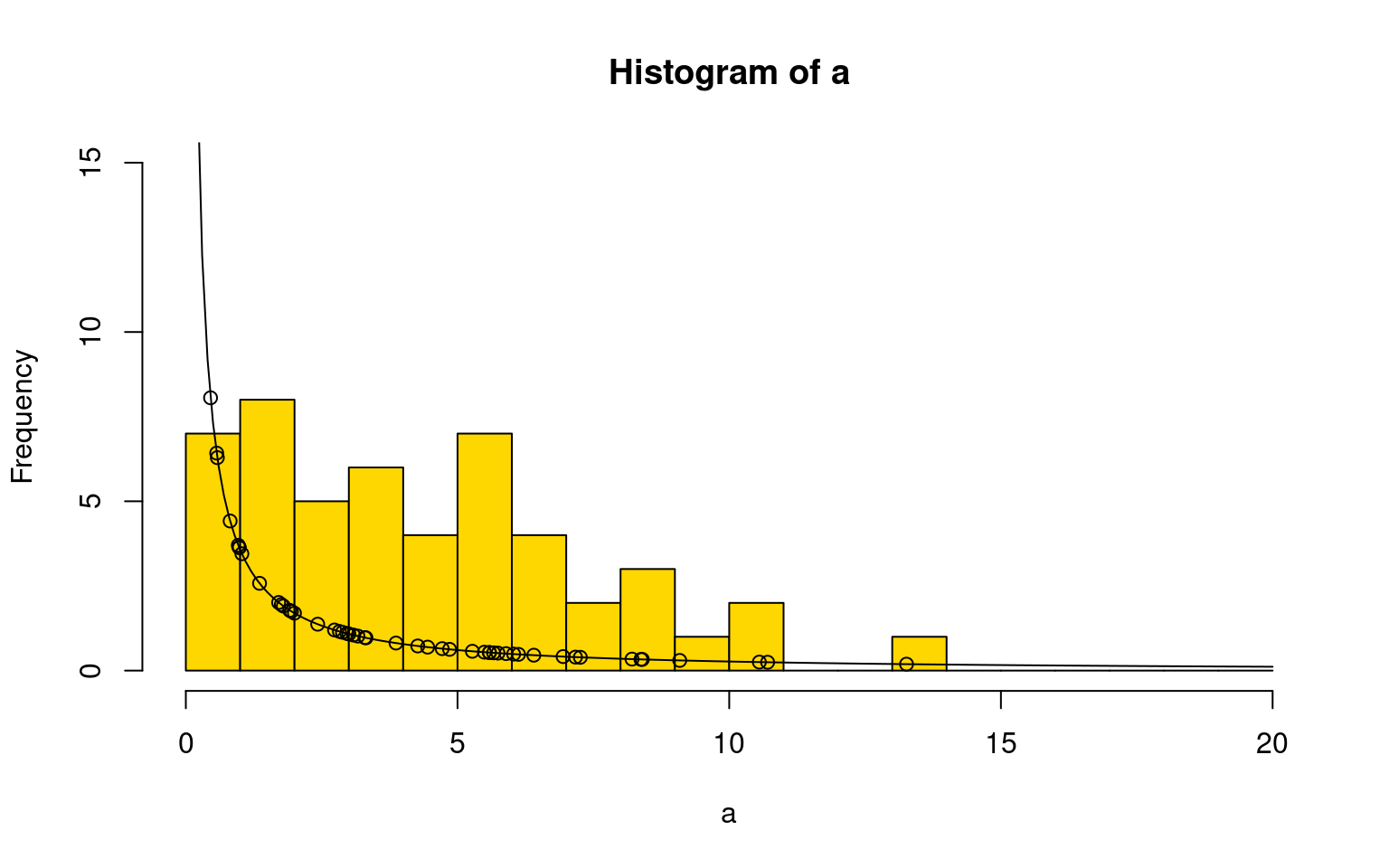

Using the same parameter search we did before, we can hone in on a region that maximimizes likelihood:

shapes <- seq(1,2.5,.1)
scales <- seq(.5,10,.5)
loglikes <- matrix(NA, nrow=length(shapes),ncol=length(scales))
for(i in 1:length(shapes))
  for(j in 1:length(scales))
  {
    loglikes[i,j] <- sum(dweibull(a,shape=shapes[i],scale=scales[j],log=TRUE))
  }

matplot(shapes,loglikes,type="l",lty=1,col="black", ylim=c(-250,0))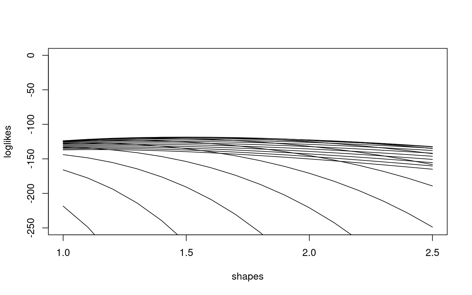

maxshape <-shapes[which(rowSums(loglikes==max(loglikes))==1)]
maxscale <- scales[which(colSums(loglikes==max(loglikes))==1)]
print(paste("Shape: ",maxshape))

[1] "Shape:  1.5"

print(paste("scale: ",maxscale))

[1] "scale:  5"

hist(a,breaks=0:20,ylim=c(0,15),col="gold",main=paste("Shape: ",maxshape,"\nscale:",maxscale))
points(0:200/10,dweibull(0:200/10,maxshape,maxscale)*50,type="l")
points(a,dweibull(a,maxshape,maxscale)*50)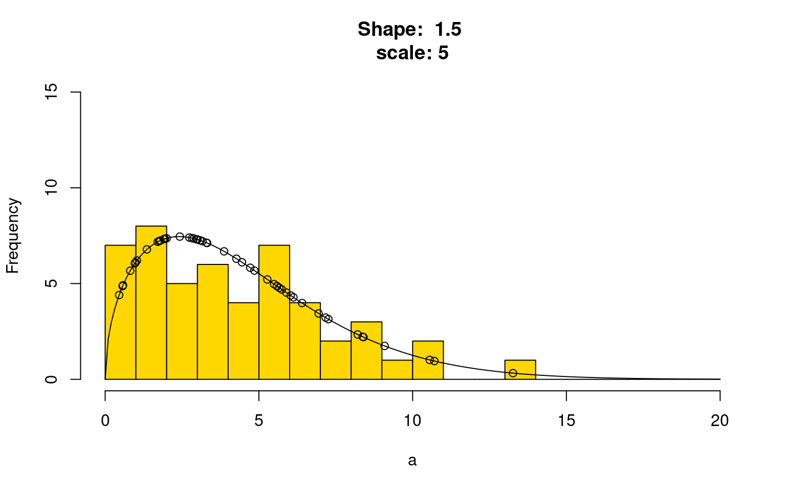

For many distributions, there are better ways of estimating the maximum likelihood parameters than grid-search. In fact, we tend to choose theoretical distributions whose maximum likelihood parameters are easy to estimate. However, the estimation process typically requires iterative numerical estimation of the values in a way that is proved to converge to the best estimate. We don’t usually have to worry about this– it is implemented behind the scenes in the glm() function in R generalized least models, using using an iterative weighted least squares process. So before we cover glm, let’s briefly consider weighted least squares.

Weighted Least Squares

One way we can extend the OLS model is to consider weighted regression. Sometimes, to create a better, more predictive, or more representative model, we might want to weigh some values more than others. Consider the state.x77 data set:

head(state.x77)

           Population Income Illiteracy Life Exp Murder HS Grad Frost   Area
Alabama          3615   3624        2.1    69.05   15.1    41.3    20  50708
Alaska            365   6315        1.5    69.31   11.3    66.7   152 566432
Arizona          2212   4530        1.8    70.55    7.8    58.1    15 113417
Arkansas         2110   3378        1.9    70.66   10.1    39.9    65  51945
California      21198   5114        1.1    71.71   10.3    62.6    20 156361
Colorado         2541   4884        0.7    72.06    6.8    63.9   166 103766

Suppose we want to compute whether murder rate can be predicted based on income, illiteracy, and high school graduation rate

state <- as.data.frame(state.x77)
colnames(state)[c(4,6)] <- c("LifeExp","HS") 
state$name <- rownames(state)
model1 <- lm(Murder~Income+Illiteracy+HS,data=state)
summary(model1)


Call:
lm(formula = Murder ~ Income + Illiteracy + HS, data = state)

Residuals:
    Min      1Q  Median      3Q     Max 
-6.0348 -1.7922  0.1427  1.5711  6.9795 

Coefficients:
              Estimate Std. Error t value Pr(>|t|)    
(Intercept)  1.7936267  4.3865984   0.409    0.685    
Income       0.0009038  0.0007918   1.141    0.260    
Illiteracy   4.1229869  0.8309778   4.962    1e-05 ***
HS          -0.0611705  0.0718824  -0.851    0.399    
---
Signif. codes:  0 '***' 0.001 '**' 0.01 '*' 0.05 '.' 0.1 ' ' 1

Residual standard error: 2.669 on 46 degrees of freedom
Multiple R-squared:  0.5093,    Adjusted R-squared:  0.4773 
F-statistic: 15.91 on 3 and 46 DF,  p-value: 3.103e-07

In this model, illiteracy predicts murder rate, but income and HS does not. But, states differ substantially in their population. If we consider the larger states more strongly, we can downplay the small states, which might possibly be noisier observations. We can do this by providing the weights argument:

model2 <- lm(Murder~Income+Illiteracy+HS,weights=Population,data=state)
summary(model2)


Call:
lm(formula = Murder ~ Income + Illiteracy + HS, data = state, 
    weights = Population)

Weighted Residuals:
    Min      1Q  Median      3Q     Max 
-363.70  -80.86  -29.02   46.77  341.46 

Coefficients:
              Estimate Std. Error t value Pr(>|t|)    
(Intercept) -0.7255219  4.7203120  -0.154   0.8785    
Income       0.0020790  0.0009418   2.207   0.0323 *  
Illiteracy   4.4116511  0.8536518   5.168 4.99e-06 ***
HS          -0.1060555  0.0768549  -1.380   0.1743    
---
Signif. codes:  0 '***' 0.001 '**' 0.01 '*' 0.05 '.' 0.1 ' ' 1

Residual standard error: 154 on 46 degrees of freedom
Multiple R-squared:  0.5179,    Adjusted R-squared:  0.4864 
F-statistic: 16.47 on 3 and 46 DF,  p-value: 2.08e-07

We can see that now, income matters. It is hard to understand why, so let’s look at some scatterplots:

library(GGally)
library(dplyr)
ggpairs(dplyr::select(state,Murder,Population,Income, Illiteracy,HS),progress=F)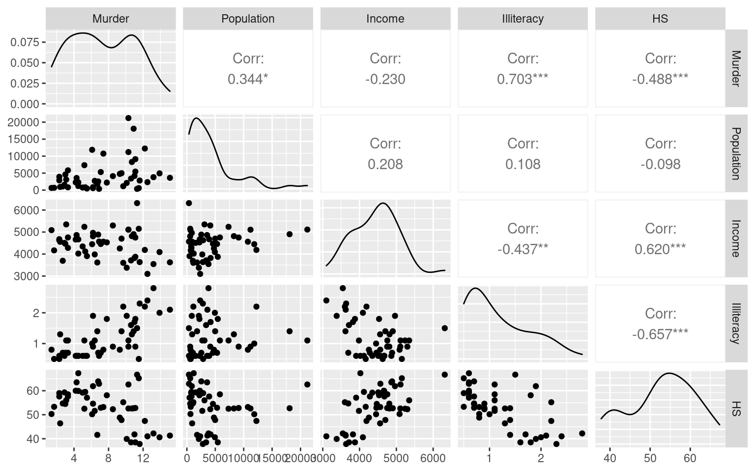

These show correlations between Murder rate and income might be impacted by an outlier. We can make the size of the point scale to population size, to see why the weighted model might be doing better:

library(ggplot2)
library(ggrepel)

ggplot(state,aes(x=Income,y=Murder,size=Population)) + geom_point() + geom_text_repel(aes(label=name))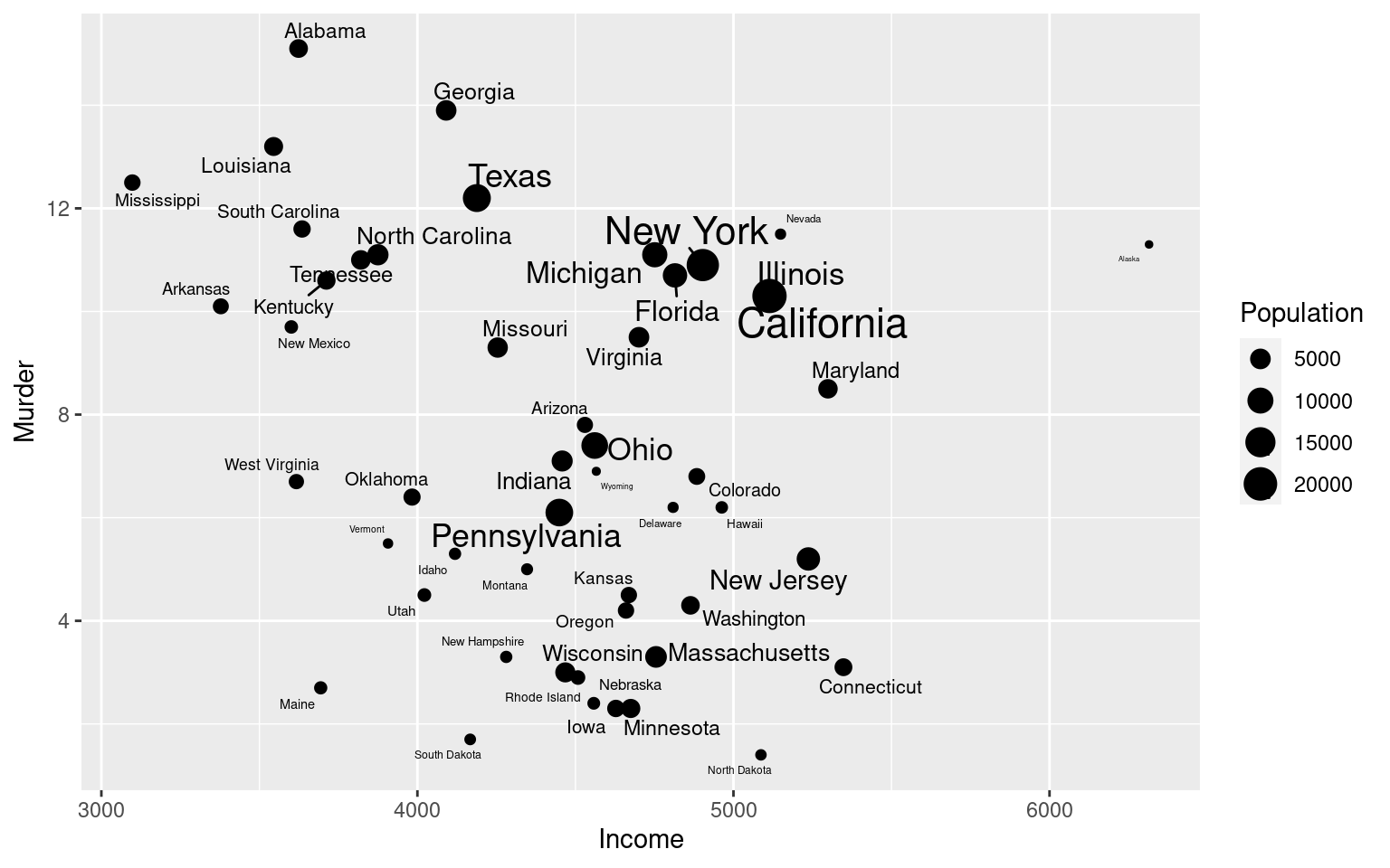

 cor(state$Income,state$Murder)

[1] -0.2300776

Notice how when all states are equally weighted, we don’t see a significant relationship between income and Murder rate. Maybe this is unfair because some states are much larger than others. If we force the deviations for the larger states to have a larger impact, we see a significant (positive) relationship. Notice that the primary relationship between income and murder rate is negative, but this is fighting against a very strong impact of illiteracy–once illiteracy is considered, there was a positive relationship between murder rate and income. This is difficult to interpret completely, because it might alternately be reasonable to include population as a predictor.

Generalized Linear Regression

Many times, we can suspect from first principles that an ordinary linear regression model will be incorrect, mainly because of the type of outcome/response data we are trying to fit. For example, if your outcome is all ‘true’ or ‘false’, regardless of how your model is made, the errors will all be one of two values–definitely not normally distributed. If we adapt three things about the ‘ordinary least squares’ linear regression model, we can have a lot more flexibility while maintaining reasonable understanding of the relationship.

Use Maximum likelihood instead of minimize residuals
Permit transforms of the outcome variable (called a ‘link’ function)
Allow exponential-family error distributions to permit non-normal residuals.

So, instead of the ‘ordinary least squares’ regression model:

\(y = \beta_0 + \beta_1*x_1 + \beta_2*x_2 ... \beta_n*x_n + \epsilon\) where \(\epsilon ~ N(0,\sigma^2)\) (i.e., the errors are normally distributed)

we have

\(G(y) = \beta_0 + \beta_1*x_1 + \beta_2*x_2 ... \beta_n*x_n + \epsilon\)

where \(\epsilon\), the error distribution, can take be any exponential-family dsitribution (including normal, poisson, binomial, and others). Nelder and Wedderburn (1972), who demonstrated how #1 could be used to estimate parameters for when #2 and #3 are adopted, are often credited as introducing and popularizing the notion. In fact, one of the major contributions was showing how weighted least squares could be used iteratively to obtain the maximum likelihood estimate. An slight alternative used by glm in R is called Fisher’s Scoring iterations, which are reported in the output. So, the slight downside of the glm is it can no longer be estimated directly with simple statistics, but it can be estimated numerically using methods a few rounds of regression. Thus, computationally it is typically a little slower than normal regression, but unless you have very large data sets it probably won’t make much of a difference.

McCullagh and Nelder (1989) are one of the most comprehensive books on the topic. Because the GLM uses Maximimum Likelihood, it adopts a a generalized notion of variance called `deviance’ which is defined as \(-2L_{max}\). Nelder makes generalizations to the analysis of variance procedures called analysis of deviance. However, you should recognize that deviance, if adjusted appropriately using the number of parameters to penalize for model complexity, becomes the AIC information metric (and the BIC if also adjusted for the number of observations.)

Generalized Linear Regression as linear regression.

If the link function is the “identity” function \(f(x)=x\) and the error distribution is guassian/normal, we get ordinary least squares (albeit estimated with maximum likeliood)

x <-matrix(runif(40),ncol=4) 
y <-  3 + x %*% c(-1,3.5, 2.2, -4) + rnorm(10)*2

summary(lm(y~x))


Call:
lm(formula = y ~ x)

Residuals:
      1       2       3       4       5       6       7       8       9      10 
 0.7053  0.0520  0.4624  0.7057  0.1534  1.5362 -1.1861 -0.6531  1.0663 -2.8421 

Coefficients:
            Estimate Std. Error t value Pr(>|t|)  
(Intercept)   4.9987     2.3748   2.105   0.0892 .
x1            0.2414     2.7413   0.088   0.9332  
x2            2.0817     2.0804   1.001   0.3630  
x3            1.7618     2.0736   0.850   0.4343  
x4           -6.4381     2.1898  -2.940   0.0323 *
---
Signif. codes:  0 '***' 0.001 '**' 0.01 '*' 0.05 '.' 0.1 ' ' 1

Residual standard error: 1.711 on 5 degrees of freedom
Multiple R-squared:  0.7827,    Adjusted R-squared:  0.6088 
F-statistic: 4.502 on 4 and 5 DF,  p-value: 0.06509

summary(glm(y~x,family=gaussian()))


Call:
glm(formula = y ~ x, family = gaussian())

Deviance Residuals: 
      1        2        3        4        5        6        7        8  
 0.7053   0.0520   0.4624   0.7057   0.1534   1.5362  -1.1861  -0.6531  
      9       10  
 1.0663  -2.8421  

Coefficients:
            Estimate Std. Error t value Pr(>|t|)  
(Intercept)   4.9987     2.3748   2.105   0.0892 .
x1            0.2414     2.7413   0.088   0.9332  
x2            2.0817     2.0804   1.001   0.3630  
x3            1.7618     2.0736   0.850   0.4343  
x4           -6.4381     2.1898  -2.940   0.0323 *
---
Signif. codes:  0 '***' 0.001 '**' 0.01 '*' 0.05 '.' 0.1 ' ' 1

(Dispersion parameter for gaussian family taken to be 2.928703)

    Null deviance: 67.384  on 9  degrees of freedom
Residual deviance: 14.644  on 5  degrees of freedom
AIC: 44.193

Number of Fisher Scoring iterations: 2

Notice how the estimates of parameter values are the same, but now we get ‘deviance’. Deviance is related to the log-likelihood of the data, rather than the sum-squared error.

Modeling counts data: Poisson Generalized Linear Regression

Consider data that are counts–usually small whole numbers. For example, you may have a large epidemiological study with 10,000 enrollees; half of whom took a vaccine to prevent an infection that leads to cancer, and another half who did not. At the end of the day, you may have 25 people in the control group, in comparison to 13 in the vaccine group, who were diagnosed with the cancer after 5 years. Did the treatment have an effect? It appears to have reduced the incidence of a low-probability event by about half, which would be great if you could have identified who the twelve people were saved and just give the vaccine to them.

A standard regression model might be fine here, but there are a few reasons why you might entertain a glm. First, counts have a lower value of 0, and can only take on whole numbers–two ways the normal error distribution may be violated. However, the Poisson distribution is designed for this sort of data–it is a discrete distribution predicting the number of times an event would occur given a known rate of occurrence. Also, counts are ratio-scaled, so that a value twice as large as another has a real meaning. This implies a logarithmic transform (link) is reasonable. For , example, suppose you found that women were twice as likely to get the disease as men. You might assume that the treatment would reduce the impact of the disease by 50% in both men and women, which is a linear effect on log(incidence), or a log-link function.

As a worked example, consider the FIFI World Cup data set described in the following paper: http://www.public.iastate.edu/~curleyb/research.html

Here, they collected statistics from FIFA World Cup matches dating back to 1930. Let’s consider the total number of yellow and red cards issued over time. This is the sum of three columns.

wc <- read.csv("world_cup.csv")
head(wc)

  X Year Winners Runnersup    Team MP GF GA PEN SOG SW FKR OFF CK W D L Y YCR R
1 1 1930 Uruguay Argentina Romania  2  3  5   0   3  0   0   0  0 1 0 1 0   0 0
2 2 1930 Uruguay Argentina Uruguay  4 15  3   0  15  0   0   0  0 4 0 0 0   0 0
3 3 1930 Uruguay Argentina     USA  3  7  6   0   7  0   0   0  0 2 0 1 0   0 0
  FC FS     Loc
1  0  0 Uruguay
2  0  0 Uruguay
3  0  0 Uruguay
 [ reached 'max' / getOption("max.print") -- omitted 3 rows ]

wc$Cards <- wc$Y + wc$YCR + wc$R

According to the data description, the columns are

Team
MP = matches played,
GF = goals for,
GA = goals against,
PEN = penalty goals
SOG = shots on goal,
SW = shots wide,
FKR = free kicks received,
OFF = offsides,
CK = corner kicks,
W = wins,
D = draws,
L = losses,
Y = yellow cards,
YCR = second yellow card and red card,
R = red card,
FC= fouls committed,
FS = fouls suffered,
Year =year of world cup,
Loc =host nation.

To predict cards given, maybe we want to see whether players are more likely to behave badly in response to game situations and rule violations. We can compute the end total points and margin of victory, and also use number of offsides, fouls committed, and fouls against. We will start with a normal linear regression, using a polynomial of power 3 for to capture the non-linear increase over time. So far, this is just a standard linear regression. Because each team played different numbers of matches, we will include MP as a predictor as well.

wc$margin <- wc$GF-wc$GA
wc$total <- wc$GF+wc$GA

model <- lm(Cards~poly(Year,3)+ margin + total+SOG+OFF+FC+FS+MP,data=wc)

wc$fit1 <- model$fitted.values

ggplot(wc,aes(x=Year,y=Cards))+geom_point()+geom_jitter() + 
   geom_point(aes(x=Year,y=fit1),colour="gold",size=2) + theme_bw()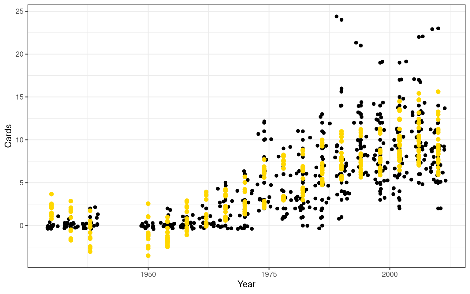

summary(model)


Call:
lm(formula = Cards ~ poly(Year, 3) + margin + total + SOG + OFF + 
    FC + FS + MP, data = wc)

Residuals:
    Min      1Q  Median      3Q     Max 
-6.7512 -1.6636 -0.1297  1.5785 13.0192 

Coefficients:
                 Estimate Std. Error t value Pr(>|t|)    
(Intercept)     -0.301165   0.521798  -0.577 0.564167    
poly(Year, 3)1  48.458972   3.841580  12.614  < 2e-16 ***
poly(Year, 3)2  14.776361   3.779787   3.909 0.000110 ***
poly(Year, 3)3 -20.853706   2.923430  -7.133 4.95e-12 ***
margin          -0.066949   0.041679  -1.606 0.109032    
total           -0.048703   0.035884  -1.357 0.175506    
SOG             -0.003364   0.042459  -0.079 0.936885    
OFF              0.144979   0.052685   2.752 0.006209 ** 
FC               0.072045   0.017726   4.064 5.85e-05 ***
FS              -0.074276   0.019474  -3.814 0.000159 ***
MP               1.436937   0.161776   8.882  < 2e-16 ***
---
Signif. codes:  0 '***' 0.001 '**' 0.01 '*' 0.05 '.' 0.1 ' ' 1

Residual standard error: 2.542 on 382 degrees of freedom
Multiple R-squared:  0.727, Adjusted R-squared:  0.7199 
F-statistic: 101.7 on 10 and 382 DF,  p-value: < 2.2e-16

Overall, the model fits reasonably well (\(R^2=.73\)). Furthermore, most of the predictors are significant, indicating that total points and shots-on-goal are marginally predictive, but offsides and other fouls really are predictive of this ‘bad behavior’ warnings.

Next, let’s fit this as a glm. Here, the model is identical, but we specify family=poisson. We don’t need to specify the link as log here, because that is the default, but we did anyway. By specifying a poisson/log link, we are trying to model a couple things:

Note that in the original, predicted values are sometimes less than 0. A poisson model does not allow negative values.
Note that the effect of any predictor on penalties is the same, regardless of era. So, the FC cost increases penalty cards the same amount (.07 per FC) as much in 1930 as it does in 2000, when 5 times as many cards are being given. A log-link will make this impact proportional instead of linear.

model2 <- glm(Cards~poly(Year,3)+margin+total+SOG+OFF+FC+FS+ MP,
              family=poisson(link="log"),data=wc)
wc$fitted <- model2$fitted.values

ggplot(wc,aes(x=Year,y=Cards))+geom_point()+geom_jitter()+
   geom_point(aes(x=Year,y=fitted),colour="gold",size=2) + theme_bw()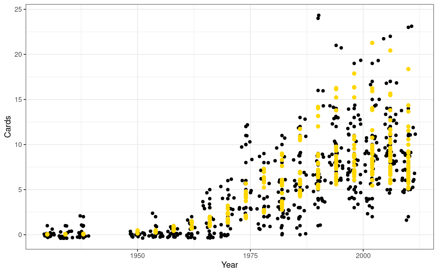

summary(model2)


Call:
glm(formula = Cards ~ poly(Year, 3) + margin + total + SOG + 
    OFF + FC + FS + MP, family = poisson(link = "log"), data = wc)

Deviance Residuals: 
    Min       1Q   Median       3Q      Max  
-3.0008  -0.8130  -0.2922   0.4790   2.7255  

Coefficients:
                Estimate Std. Error z value Pr(>|z|)    
(Intercept)    -0.187758   0.118927  -1.579 0.114390    
poly(Year, 3)1 29.903500   2.705644  11.052  < 2e-16 ***
poly(Year, 3)2 -6.564833   2.209660  -2.971 0.002969 ** 
poly(Year, 3)3 -3.190207   1.052523  -3.031 0.002437 ** 
margin         -0.007400   0.007405  -0.999 0.317658    
total          -0.003028   0.006677  -0.454 0.650177    
SOG            -0.013184   0.005474  -2.409 0.016012 *  
OFF             0.011906   0.006401   1.860 0.062892 .  
FC              0.009590   0.002311   4.150 3.32e-05 ***
FS             -0.008521   0.002468  -3.453 0.000555 ***
MP              0.290236   0.028413  10.215  < 2e-16 ***
---
Signif. codes:  0 '***' 0.001 '**' 0.01 '*' 0.05 '.' 0.1 ' ' 1

(Dispersion parameter for poisson family taken to be 1)

    Null deviance: 1998.89  on 392  degrees of freedom
Residual deviance:  402.29  on 382  degrees of freedom
AIC: 1464.9

Number of Fisher Scoring iterations: 6

cor(wc$fitted,wc$Cards)^2

[1] 0.782944

In this case, the results are fairly similar (\(R^2=.78\)), except SOG/OFF are no longer significant but margin and total are. This happens in part because these predictors all impact the total number of cards as a proportion of baseline, not as an additive value. So, margin and total impact the proportion of red cards, allowing them to have very small impact back when no cards were given, but when 10-15 cards are given per team in the tournament, these might impact by a larger margin. But the fit looks more reasonable, especially at the low end, where our normal regression made predictions of negative values.

Deviance and Comparing Models

The Null deviance is like the total residual error for the intercept-only model, and “Residual deviance” is like the RSE for the current model. We can examine and compare models usung these deviance scores, or via the AIC (because this uses likelihood). Suppose we want to see if a 4th order polynomial is better:

model2b <- glm(Cards~poly(Year,4)+margin+total+SOG+OFF+FC+FS+MP,
              family=poisson(link="log"),data=wc)
summary(model2b)


Call:
glm(formula = Cards ~ poly(Year, 4) + margin + total + SOG + 
    OFF + FC + FS + MP, family = poisson(link = "log"), data = wc)

Deviance Residuals: 
    Min       1Q   Median       3Q      Max  
-3.0664  -0.7928  -0.3339   0.4942   2.6597  

Coefficients:
                Estimate Std. Error z value Pr(>|z|)    
(Intercept)    -0.156093   0.114679  -1.361 0.173470    
poly(Year, 4)1 28.688130   2.363128  12.140  < 2e-16 ***
poly(Year, 4)2 -4.771263   2.064681  -2.311 0.020839 *  
poly(Year, 4)3 -5.246592   1.473707  -3.560 0.000371 ***
poly(Year, 4)4  1.486073   0.870747   1.707 0.087885 .  
margin         -0.006437   0.007416  -0.868 0.385397    
total          -0.001479   0.006747  -0.219 0.826443    
SOG            -0.013615   0.005484  -2.483 0.013040 *  
OFF             0.011775   0.006394   1.842 0.065546 .  
FC              0.009787   0.002311   4.236 2.28e-05 ***
FS             -0.008227   0.002472  -3.327 0.000876 ***
MP              0.281877   0.028818   9.781  < 2e-16 ***
---
Signif. codes:  0 '***' 0.001 '**' 0.01 '*' 0.05 '.' 0.1 ' ' 1

(Dispersion parameter for poisson family taken to be 1)

    Null deviance: 1998.89  on 392  degrees of freedom
Residual deviance:  399.46  on 381  degrees of freedom
AIC: 1464.1

Number of Fisher Scoring iterations: 6

AIC(model2)

[1] 1464.896

AIC(model2b)

[1] 1464.064

anova(model2, model2b,test="Chisq")

Analysis of Deviance Table

Model 1: Cards ~ poly(Year, 3) + margin + total + SOG + OFF + FC + FS + 
    MP
Model 2: Cards ~ poly(Year, 4) + margin + total + SOG + OFF + FC + FS + 
    MP
  Resid. Df Resid. Dev Df Deviance Pr(>Chi)  
1       382     402.29                       
2       381     399.46  1   2.8319  0.09241 .
---
Signif. codes:  0 '***' 0.001 '**' 0.01 '*' 0.05 '.' 0.1 ' ' 1

Deviance is often compared using a Chi-squared test, although the AIC measure is also appropriate. Here, the model2b has the lower AIC (just barely), but it is not significantly better than the smaller model according to a chi-squared test. Now, could we test specifically whether SOG matters? Let’s remove it from the model and compare the two.

model2c <- glm(Cards~poly(Year,4)+margin+total+OFF+FC+FS+MP,
              family=poisson(link="log"),data=wc)
summary(model2c)


Call:
glm(formula = Cards ~ poly(Year, 4) + margin + total + OFF + 
    FC + FS + MP, family = poisson(link = "log"), data = wc)

Deviance Residuals: 
    Min       1Q   Median       3Q      Max  
-3.0958  -0.8037  -0.3454   0.5121   2.6896  

Coefficients:
                Estimate Std. Error z value Pr(>|z|)    
(Intercept)    -0.092966   0.111606  -0.833 0.404854    
poly(Year, 4)1 28.571829   2.380926  12.000  < 2e-16 ***
poly(Year, 4)2 -5.184181   2.078965  -2.494 0.012644 *  
poly(Year, 4)3 -5.192876   1.482706  -3.502 0.000461 ***
poly(Year, 4)4  1.386069   0.870537   1.592 0.111340    
margin         -0.012661   0.006957  -1.820 0.068757 .  
total          -0.007269   0.006286  -1.156 0.247532    
OFF             0.010880   0.006404   1.699 0.089352 .  
FC              0.009473   0.002285   4.145 3.40e-05 ***
FS             -0.010792   0.002231  -4.838 1.31e-06 ***
MP              0.260987   0.027417   9.519  < 2e-16 ***
---
Signif. codes:  0 '***' 0.001 '**' 0.01 '*' 0.05 '.' 0.1 ' ' 1

(Dispersion parameter for poisson family taken to be 1)

    Null deviance: 1998.89  on 392  degrees of freedom
Residual deviance:  405.66  on 382  degrees of freedom
AIC: 1468.3

Number of Fisher Scoring iterations: 6

AIC(model2b)

[1] 1464.064

AIC(model2c)

[1] 1468.263

anova(model2b,model2c,test="Chisq")

Analysis of Deviance Table

Model 1: Cards ~ poly(Year, 4) + margin + total + SOG + OFF + FC + FS + 
    MP
Model 2: Cards ~ poly(Year, 4) + margin + total + OFF + FC + FS + MP
  Resid. Df Resid. Dev Df Deviance Pr(>Chi)  
1       381     399.46                       
2       382     405.66 -1  -6.1991  0.01278 *
---
Signif. codes:  0 '***' 0.001 '**' 0.01 '*' 0.05 '.' 0.1 ' ' 1

Removing SOG makes a significant difference according to the \(\chi^2\) test, and the AIC value is larger/worse (1468 vs 1464). Both of these tell us that SOG matter, because removing it makes for a significantly worse model.

Interpreting parameters

In the Poisson model, the parameter estimates are interpretable in terms of their impact on the log-outcome.

\(log(y) = \beta_0 + \beta_1 x_1 + \beta_2 x_2 ...\)

Which implies:

\(y = exp(\beta_0 + \beta_1 x_1 + \beta_2 x_2 ...)\)

\(y = exp(\beta_0) \exp({\beta_1 x_1}) \exp({\beta_2 x_2})...\)

You can see how y is the product of each \(\beta x\) term exponentiated. But since the \(\beta\) values are available, we can re-write this as each \(exp({\beta})\) value raised to the \(x_i\) power. Focusing on just a few of the parameters:

\(y = exp(.49) \times exp(.02386)^{margin} \times exp(.0287)^{total}\)

Calculating each exponential, we get:

\(y = 1.63 \times 1.023^{margin} \times 1.029^{total} ...\)

This suggests that for each unit of total, the card rate increases by 2.9%; and for each point difference between winner and loser the card rate increases by 2.3%. Notice that prior to tranform, the beta weight is approximately equal to the the transformed rate -1.0. For small values, this is a well-known engineering approximation; for large values such as the intercept (.49), this no longer holds well (.49 vs .63).

Overdispersion

On important diagnostic of the GLM is to know whether the deviance is too large. The rule of thumb is that deviance should generally be about the same as the number of the residual degrees of freedom. If it is substantially larger, we should consider a better model, a different model, or accounting for the so-called over-dispersion directly. There are many resources for determining how to deal with this.

In general, the quasi- models allow for fitting of an overdispersion parameter. With the over-dispersion model, we can force the dispersion parameter to 1 (no overdispersion) to see if it makes a difference. A larger value means that the variance has more variability than you would expect if the assumptions were correct.

model.od <- glm(Cards~poly(Year,3)+margin+total+FC+FS,
              family=quasipoisson(link="log"),data=wc)
summary(model.od)


Call:
glm(formula = Cards ~ poly(Year, 3) + margin + total + FC + FS, 
    family = quasipoisson(link = "log"), data = wc)

Deviance Residuals: 
    Min       1Q   Median       3Q      Max  
-3.2118  -0.9223  -0.2312   0.3917   4.9898  

Coefficients:
                 Estimate Std. Error t value Pr(>|t|)    
(Intercept)      0.437036   0.147188   2.969 0.003172 ** 
poly(Year, 3)1  34.317515   4.210008   8.151 5.11e-15 ***
poly(Year, 3)2 -11.863598   3.393383  -3.496 0.000527 ***
poly(Year, 3)3  -2.390839   1.582698  -1.511 0.131708    
margin           0.024944   0.007587   3.288 0.001103 ** 
total            0.028369   0.006700   4.234 2.87e-05 ***
FC               0.011364   0.003037   3.741 0.000211 ***
FS              -0.008862   0.002924  -3.030 0.002608 ** 
---
Signif. codes:  0 '***' 0.001 '**' 0.01 '*' 0.05 '.' 0.1 ' ' 1

(Dispersion parameter for quasipoisson family taken to be 1.747136)

    Null deviance: 1998.89  on 392  degrees of freedom
Residual deviance:  508.37  on 385  degrees of freedom
AIC: NA

Number of Fisher Scoring iterations: 6

anova(model.od,test="Chisq")

Analysis of Deviance Table

Model: quasipoisson, link: log

Response: Cards

Terms added sequentially (first to last)

              Df Deviance Resid. Df Resid. Dev  Pr(>Chi)    
NULL                            392    1998.89              
poly(Year, 3)  3  1361.54       389     637.35 < 2.2e-16 ***
margin         1    71.34       388     566.02 1.661e-10 ***
total          1    31.25       387     534.77 2.346e-05 ***
FC             1    10.12       386     524.65   0.01611 *  
FS             1    16.28       385     508.37   0.00227 ** 
---
Signif. codes:  0 '***' 0.001 '**' 0.01 '*' 0.05 '.' 0.1 ' ' 1

anova(model.od,dispersion=1,test="Chisq")

Analysis of Deviance Table

Model: quasipoisson, link: log

Response: Cards

Terms added sequentially (first to last)

              Df Deviance Resid. Df Resid. Dev  Pr(>Chi)    
NULL                            392    1998.89              
poly(Year, 3)  3  1361.54       389     637.35 < 2.2e-16 ***
margin         1    71.34       388     566.02 < 2.2e-16 ***
total          1    31.25       387     534.77 2.270e-08 ***
FC             1    10.12       386     524.65  0.001468 ** 
FS             1    16.28       385     508.37 5.469e-05 ***
---
Signif. codes:  0 '***' 0.001 '**' 0.01 '*' 0.05 '.' 0.1 ' ' 1

Here, the overdispersion parameter of 1.7 is a bit worrisome, but the signifance tests were all significant even when using the quasipoisson model.

Overdispersion usually indicates that you have additional variability in your data set than the GLM error model supposes. This is a bit strange thinking about when we considering a normal distribution, but for specific distributions, the variability of the data suggest essentially that the data could not have arisen from a single parameter value. An example might be that a basketball team’s number of three-point attempts leads to a poisson model that has over-dispersion, which may be because different members of the team are responsible for different proportions of the shots, and these players are impacted by different other factors, leading to a data distribution that does not fit the poisson model well. A Bayesian inference approach is another alternative to handling this issue.

For example, in the world cup data, different teams played different numbers of matches. In model.od, I did not include MP, and that might be a source of variability that does not easily map onto tho poisson distribution. Let’s add it back in and see what happens:

model.od <- glm(Cards~poly(Year,3)+margin+total+FC+FS+MP,
              family=quasipoisson(link="log"),data=wc)
summary(model.od)


Call:
glm(formula = Cards ~ poly(Year, 3) + margin + total + FC + FS + 
    MP, family = quasipoisson(link = "log"), data = wc)

Deviance Residuals: 
    Min       1Q   Median       3Q      Max  
-3.0220  -0.8252  -0.2898   0.5212   2.7344  

Coefficients:
                Estimate Std. Error t value Pr(>|t|)    
(Intercept)    -0.127879   0.126362  -1.012  0.31217    
poly(Year, 3)1 29.804019   2.951869  10.097  < 2e-16 ***
poly(Year, 3)2 -6.886981   2.410574  -2.857  0.00451 ** 
poly(Year, 3)3 -3.230715   1.149921  -2.810  0.00522 ** 
margin         -0.012290   0.007563  -1.625  0.10496    
total          -0.007834   0.006806  -1.151  0.25046    
FC              0.010101   0.002460   4.106 4.93e-05 ***
FS             -0.009969   0.002373  -4.201 3.30e-05 ***
MP              0.267802   0.029378   9.116  < 2e-16 ***
---
Signif. codes:  0 '***' 0.001 '**' 0.01 '*' 0.05 '.' 0.1 ' ' 1

(Dispersion parameter for quasipoisson family taken to be 1.196072)

    Null deviance: 1998.89  on 392  degrees of freedom
Residual deviance:  411.07  on 384  degrees of freedom
AIC: NA

Number of Fisher Scoring iterations: 6

anova(model.od,test="Chisq")

Analysis of Deviance Table

Model: quasipoisson, link: log

Response: Cards

Terms added sequentially (first to last)

              Df Deviance Resid. Df Resid. Dev  Pr(>Chi)    
NULL                            392    1998.89              
poly(Year, 3)  3  1361.54       389     637.35 < 2.2e-16 ***
margin         1    71.34       388     566.02 1.138e-14 ***
total          1    31.25       387     534.77 3.198e-07 ***
FC             1    10.12       386     524.65  0.003632 ** 
FS             1    16.28       385     508.37  0.000225 ***
MP             1    97.31       384     411.07 < 2.2e-16 ***
---
Signif. codes:  0 '***' 0.001 '**' 0.01 '*' 0.05 '.' 0.1 ' ' 1

anova(model.od,dispersion=1,test="Chisq")

Analysis of Deviance Table

Model: quasipoisson, link: log

Response: Cards

Terms added sequentially (first to last)

              Df Deviance Resid. Df Resid. Dev  Pr(>Chi)    
NULL                            392    1998.89              
poly(Year, 3)  3  1361.54       389     637.35 < 2.2e-16 ***
margin         1    71.34       388     566.02 < 2.2e-16 ***
total          1    31.25       387     534.77 2.270e-08 ***
FC             1    10.12       386     524.65  0.001468 ** 
FS             1    16.28       385     508.37 5.469e-05 ***
MP             1    97.31       384     411.07 < 2.2e-16 ***
---
Signif. codes:  0 '***' 0.001 '**' 0.01 '*' 0.05 '.' 0.1 ' ' 1

Now, the dispersion parameter is close to 1 (1.196), which suggests that we have accounted for an important source of variability that was violating the poisson model.