Logistic Regression
Logistic Regression as a common form of the GLM
Probably the most common version of the GLM used is logistic regression. Typically, logistic regression is used to model binary outcomes, although it can essentially also model probabilities between 0 and 1, because its goal is to estimate parameters interpretable in terms of probabilities.
Logistic regression consists of:
The logistic or logit function refers to the link. The logistic (logit) function is \(1/(1+exp(-x))\), and it is the inverse of log-odds: \(log(p/(1-p))\).
A binomial error distribution is the distribution of expected heads you’d get when flipping a biased coin N times. Thus, it is appropriate for any two-level distribution in which you can represent the values as 0 and 1.
Log-odds transform
Binary outcomes can be modeled with standard regression, but they are difficult to interpret. For example, we can model the the outcome of 0 or 1, but the predicted value won’t be all 0s or 1s, and typically won’t even be bounded between 0 and 1. To make a classification, we would need to come up with some (possibly ad-hoc) rule and state that any value above 0.5 should be called a 1. If we wanted to model probabilities instead of just 0/1 values, we arrive at a similar problem–there is no guarantee that the model will produce estimates bounded within [0,1]. This is disturbing, because you could have a reasonably good model that predicts your chance of something happening is less than 0, or greater than 1.
One way to deal with this is to model the odds, which is \(p/(1-p)\). Now, there is no upper bound–as we get close to p=1.0, odds approaches INF. But there are problems as well: as p gets close to 0, odds also approaches 0, so it is bounded. Furthermore, probabilities less than 0.5 are not symmetric with probabilities above 0.5. A log transform of odds fixes both of these issues (see second figure).
library(ggplot2)
p <- 0:100/100
odds <- p/(1 - p)
logodds <- log(odds)
df <- data.frame(p, odds, logodds)
ggplot(df, aes(x = p, y = odds)) + geom_line() + ggtitle("p versus odds(p)") + theme_bw()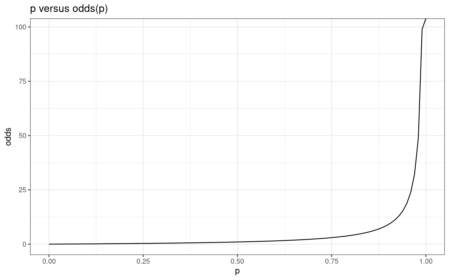
ggplot(df, aes(x = p, y = logodds)) + geom_line() + ggtitle("p versus logodds(p)") +
    theme_bw()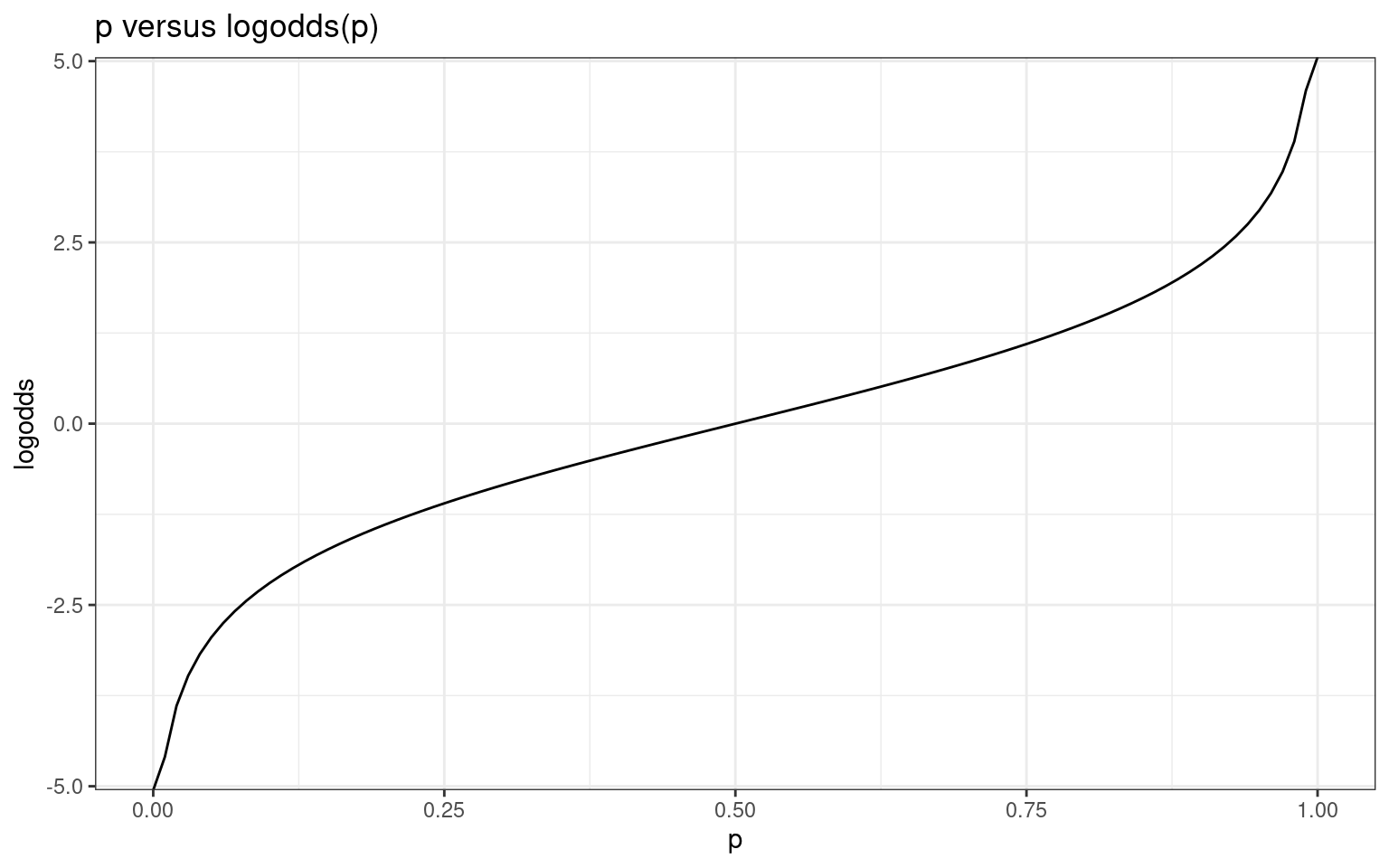
This gives a way of modeling a family of relationships between a continuous predictor and a binary outcome variable, by assuming that a predictor is linearly related to the log-odds (and then using this transform to convert to probability, and compute likelihood of data). By fitting the equivalent of an intercept term, we move this curve left and right. By fitting slopes with respect to a predictor, we make the curve sharper or flatter. The logistic is always symmetric around .5, and must start at 0 and go to 1.0, but otherwise is very flexible in modeling all kinds binary, probability, and two-level categorical variables.
ggplot(df, aes(x = logodds, y = p)) + geom_line() + ggtitle("logodds(p) versus p") +
    theme_bw()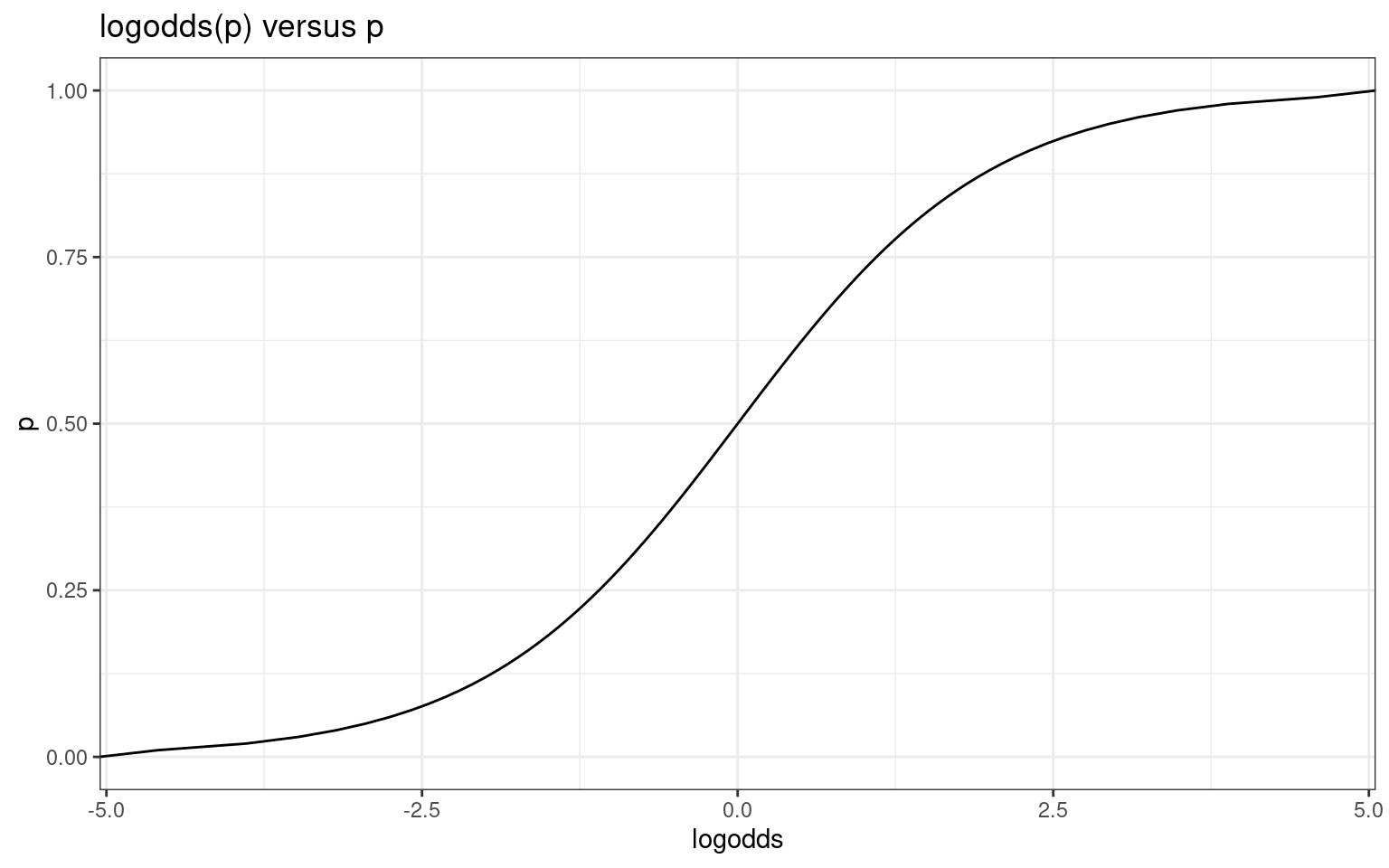
So, logistic regression transforms the outcomes so that a linear combination of predictors produces log-odds effects on the outcome. Any coefficient of the model can be transformed and interpreted as odds multiplier. This is the source of many news reports suggesting things like “smoking increases the odds of dying of cancer by X”. These results are easily interpretable by the public, and come directly from logistic regression models.
Worked Example
The birthwt data set has 130 children with a birthweight above 2.5 kilos, and 59 below, and many potential predictors. In regular regression, we might consider modeling the continuous weight value, but instead, we might want to model low birth weight, which could indicate risk. This is binary, and so is appropriate for a logistic regression. Let’s model this and see how a number of risk factors to at predicting low birth weight.
The following code estimates a logistic regression model using the glm (generalized linear model) function. Specifying the “family” of the model allows us to get the right distribution.
library(MASS)  #for birthwt data:
data(birthwt)

summary(birthwt)
low age lwt race
Min. :0.0000 Min. :14.00 Min. : 80.0 Min. :1.000
1st Qu.:0.0000 1st Qu.:19.00 1st Qu.:110.0 1st Qu.:1.000
Median :0.0000 Median :23.00 Median :121.0 Median :1.000
Mean :0.3122 Mean :23.24 Mean :129.8 Mean :1.847
3rd Qu.:1.0000 3rd Qu.:26.00 3rd Qu.:140.0 3rd Qu.:3.000
Max. :1.0000 Max. :45.00 Max. :250.0 Max. :3.000
smoke ptl ht ui
Min. :0.0000 Min. :0.0000 Min. :0.00000 Min. :0.0000
1st Qu.:0.0000 1st Qu.:0.0000 1st Qu.:0.00000 1st Qu.:0.0000
Median :0.0000 Median :0.0000 Median :0.00000 Median :0.0000
Mean :0.3915 Mean :0.1958 Mean :0.06349 Mean :0.1481
3rd Qu.:1.0000 3rd Qu.:0.0000 3rd Qu.:0.00000 3rd Qu.:0.0000
Max. :1.0000 Max. :3.0000 Max. :1.00000 Max. :1.0000
ftv bwt
Min. :0.0000 Min. : 709
1st Qu.:0.0000 1st Qu.:2414
Median :0.0000 Median :2977
Mean :0.7937 Mean :2945
3rd Qu.:1.0000 3rd Qu.:3487
Max. :6.0000 Max. :4990 table(birthwt$low)
  0   1
130  59
Note: we are leaving off the variable bwt. (This would allow us to predict perfectly.)
Build the model. Note that we don’t transform the outcome–we let the default ‘logit’ link function of the binomial family regression handle that for us.
full.model <- glm(low ~ age + lwt + factor(race) + smoke + ptl + ht + ui + ftv, data = birthwt,
    family = binomial())
summary(full.model)
Call:
glm(formula = low ~ age + lwt + factor(race) + smoke + ptl +
    ht + ui + ftv, family = binomial(), data = birthwt)

Deviance Residuals:
    Min       1Q   Median       3Q      Max
-1.8946  -0.8212  -0.5316   0.9818   2.2125

Coefficients:
               Estimate Std. Error z value Pr(>|z|)
(Intercept)    0.480623   1.196888   0.402  0.68801
age           -0.029549   0.037031  -0.798  0.42489
lwt           -0.015424   0.006919  -2.229  0.02580 *
factor(race)2  1.272260   0.527357   2.413  0.01584 *
factor(race)3  0.880496   0.440778   1.998  0.04576 *
smoke          0.938846   0.402147   2.335  0.01957 *
ptl            0.543337   0.345403   1.573  0.11571
ht             1.863303   0.697533   2.671  0.00756 **
ui             0.767648   0.459318   1.671  0.09467 .
ftv            0.065302   0.172394   0.379  0.70484
---
Signif. codes:  0 '***' 0.001 '**' 0.01 '*' 0.05 '.' 0.1 ' ' 1

(Dispersion parameter for binomial family taken to be 1)

    Null deviance: 234.67  on 188  degrees of freedom
Residual deviance: 201.28  on 179  degrees of freedom
AIC: 221.28

Number of Fisher Scoring iterations: 4
The model seems reasonable, with many of the predictors significant. Looking at the significant predictors we see last mother’s weight, race, smoking, history of hypertension are significant predictors. Weight is negative, which means that the less a mother weighs, the greater the risk of low birth weight. The others are all positive. The coefficients close to 0 have no impact on log-odds, whereas values above 0 have a positive impact, and values below 0 a negative impact–keep in mind that log-odds(.5)=0. Interpreting the results output:
- the first row reminds us what function we called
- deviance residuals is a measure of model fit
- The next table shows coefficients, std error, z statistic - all the factors are statistically significant (last column), for every one unit change in hypertension (ht) the odds of low birthweight increases by 1.749
Over-dispersion
The Logistic model assumes errors happen exactly like tossing a single coin multiple times. The coin may be biased, but we assume it is the same biased coin. But what would happen if the data were really like a jar of coins, each with a different bias? For each observation, we pick a coin and then flip it. It turns out that this would create different error distributions, and lead us to make incorrect inference. This is called over-dispersion, and it should be checked for in a logistic regression. In logistic regression, unlike in OLS, the binomial error distribution makes a strong assumption about the relationship between p and sd(p)==it should be \(\sqrt{(p*(1-p))}\). If it is not, we have an additional source of noise in the sampling.
Returning to the birth weight data, We should check for over-dispersion. If the logistic assumptions hold, residual deviance should be about the same as the degrees of freedom. If much larger, this indicates over-dispersion, and could mean we have dependencies among our data, such as you’d find in repeated-measures experiments, or variability in the sampling of people like the coin-sampling. If you are modeling accuracy in a study, and accuracy differs systematically across people, but model mean accuracy in a logistic regression, you are likely to find over-dispersion.
Let’s look at a smaller model tha involves just the significant factors:
partial.model <- glm(low ~ lwt + factor(race) + smoke + ht, data = birthwt, family = binomial())
summary(partial.model)
Call:
glm(formula = low ~ lwt + factor(race) + smoke + ht, family = binomial(),
    data = birthwt)

Deviance Residuals:
    Min       1Q   Median       3Q      Max
-1.7751  -0.8747  -0.5712   0.9634   2.1131

Coefficients:
               Estimate Std. Error z value Pr(>|z|)
(Intercept)    0.352049   0.924438   0.381  0.70333
lwt           -0.017907   0.006799  -2.634  0.00844 **
factor(race)2  1.287662   0.521648   2.468  0.01357 *
factor(race)3  0.943645   0.423382   2.229  0.02583 *
smoke          1.071566   0.387517   2.765  0.00569 **
ht             1.749163   0.690820   2.532  0.01134 *
---
Signif. codes:  0 '***' 0.001 '**' 0.01 '*' 0.05 '.' 0.1 ' ' 1

(Dispersion parameter for binomial family taken to be 1)

    Null deviance: 234.67  on 188  degrees of freedom
Residual deviance: 208.25  on 183  degrees of freedom
AIC: 220.25

Number of Fisher Scoring iterations: 4
That looks pretty good. The predictors are significant (last column). The residual deviance is a bit larger than the degrees of freedom–maybe by about 10%. But this lack of fit could come from many sources–including violations of all the same assumptions of linear regression, such as non-normal predictors, non-linearity in the predictors, etc. If we examine the only continuous predict lwt, we see some skew that might deserve a transformation, but checking this it does not impact residual variance.
A 10% higher than expected deviance is probably not unexpected, and would be fairly common to see if there was no over-dispersion (this can be tested with a chi squared test). And because the data are all binary (0/1), it would be difficult to find overdispersion. But logistic models can be used for proportions and probabilities too, and a we will see below, these can be overdispersed.
If you have large overdispersion, you may need to use a package like ‘dispmod’, which can handle a binomial overdispersed logit model. However, the package does not seem to work on this model:
library(dispmod)

partial.model1 <- glm(low ~ lwt + factor(race) + smoke + ht, data = birthwt, family = binomial())

## This dispersion model fails: glm.binomial.disp(partial.model1,verbose=T)
It will work on the example in the help, in which each case is a number of successes out several different numbers of seeds. The issue is that there are two ways of specifying the dvs of a glm logistic, either as 0/1 (which we have here), or if you have more than 1 observation per grouping, as a two column matrix with \(x\) and \((n-x)\). The dispmod wants the second kind, but with just one observation per case, you are likely to match the assumptions of the binomial model and so overdispersion would not be a problem, and the .disp model also fails here:
dv <- cbind(birthwt$low, 1 - birthwt$low)
partial.model3 <- glm(dv ~ lwt + age, data = birthwt, family = binomial(logit))
# This also does not work: glm.binomial.disp(partial.model3,verbose=T)
To fake this so we get an example that works, let’s just assume we have 2 observations per group, by multiplying everything by 2. We would not do this if we really wanted to use dispmod to estimate overdispersion for our data–we are just doing it to see what the results would have been if that were the case.
dv <- cbind(birthwt$low, 1 - birthwt$low) * 2
partial.model3 <- glm(dv ~ lwt + age, data = birthwt, family = binomial(logit))
model.od2 <- glm.binomial.disp(partial.model3, verbose = T)
Binomial overdispersed logit model fitting...
Iter.  1  phi: 1.036053
Converged after 1 iterations.
Estimated dispersion parameter: 1.036053

Call:
glm(formula = dv ~ lwt + age, family = binomial(logit), data = birthwt,
    weights = disp.weights)

Deviance Residuals:
    Min       1Q   Median       3Q      Max
-1.1251  -0.9007  -0.7413   1.3273   2.0412

Coefficients:
             Estimate Std. Error z value Pr(>|z|)
(Intercept)  1.748773   1.006012   1.738   0.0822 .
lwt         -0.012775   0.006267  -2.039   0.0415 *
age         -0.039788   0.032576  -1.221   0.2219
---
Signif. codes:  0 '***' 0.001 '**' 0.01 '*' 0.05 '.' 0.1 ' ' 1

(Dispersion parameter for binomial family taken to be 1)

    Null deviance: 230.52  on 188  degrees of freedom
Residual deviance: 223.10  on 186  degrees of freedom
AIC: 229.1

Number of Fisher Scoring iterations: 4
model.od2
Call:  glm(formula = dv ~ lwt + age, family = binomial(logit), data = birthwt,
    weights = disp.weights)

Coefficients:
(Intercept)          lwt          age
    1.74877     -0.01278     -0.03979

Degrees of Freedom: 188 Total (i.e. Null);  186 Residual
Null Deviance:      230.5
Residual Deviance: 223.1 AIC: 229.1print(paste("Dispersion parameter is:", model.od2$dispersion))[1] "Dispersion parameter is: 1.03605253501365"So, here the dispmod library estimated a specific dispersion parameter. In this case, it was not too different from 1. The dispmod library has similar overdispersion parameters for poisson and gaussian models as well.
If you did not have access to dispmod, the typical solution is to use the quasibinomial family, which also estimates a dispersion parameter for you asn well.
partial.model4 <- glm(low ~ lwt + age, data = birthwt, family = quasibinomial(logit))

summary(partial.model4)
Call:
glm(formula = low ~ lwt + age, family = quasibinomial(logit),
    data = birthwt)

Deviance Residuals:
    Min       1Q   Median       3Q      Max
-1.1352  -0.9088  -0.7480   1.3392   2.0595

Coefficients:
             Estimate Std. Error t value Pr(>|t|)
(Intercept)  1.748773   1.006043   1.738   0.0838 .
lwt         -0.012775   0.006267  -2.039   0.0429 *
age         -0.039788   0.032577  -1.221   0.2235
---
Signif. codes:  0 '***' 0.001 '**' 0.01 '*' 0.05 '.' 0.1 ' ' 1

(Dispersion parameter for quasibinomial family taken to be 1.018026)

    Null deviance: 234.67  on 188  degrees of freedom
Residual deviance: 227.12  on 186  degrees of freedom
AIC: NA

Number of Fisher Scoring iterations: 4
Here, the estimate is very close to 1.0, indicating no overdispersion, which is akin to the dispmod approach. But they do estimate different overdispersion parameters.
Comparing/Testing overall models.
Now, to find out if the overall regression is significant (not just the individual predictors) we must compare two models, just like we did with anova() to compare linear models. We can still use the anoav() function, but we cannot use the F test–we need to specify the test to use, and usually one uses a chi-squared test to compare logistic models:
full.model <- glm(low ~ age + lwt + factor(race) + smoke + ptl + ht + ui + ftv, data = birthwt,
    family = binomial())

partial.model <- glm(low ~ age + lwt + factor(race), data = birthwt, family = binomial())

anova(partial.model, full.model, test = "Chisq")
Analysis of Deviance Table
Model 1: low ~ age + lwt + factor(race)
Model 2: low ~ age + lwt + factor(race) + smoke + ptl + ht + ui + ftv
Resid. Df Resid. Dev Df Deviance Pr(>Chi)
1 184 222.66
2 179 201.28 5 21.376 0.0006877 ***
---
Signif. codes: 0 '***' 0.001 '**' 0.01 '*' 0.05 '.' 0.1 ' ' 1The result suggests that the partial model is adequate for predicting
low birth weight. Chi-Squared is not significant, so we would prefer the
smaller model. An alternative is doing a wald-test, which is available
in the lmtest and aod packages. The wald test
is essentially a t-test for individual coefficients, but we know that a
t-test on linear regression coefficients is equivalent to the F-test on
nested models.
library(lmtest)
waldtest(partial.model)
Wald test
Model 1: low ~ age + lwt + factor(race)
Model 2: low ~ 1
Res.Df Df F Pr(>F)
1 184
2 188 -4 2.6572 0.03436 *
---
Signif. codes: 0 '***' 0.001 '**' 0.01 '*' 0.05 '.' 0.1 ' ' 1waldtest(full.model)Wald test
Model 1: low ~ age + lwt + factor(race) + smoke + ptl + ht + ui + ftv
Model 2: low ~ 1
Res.Df Df F Pr(>F)
1 179
2 188 -9 2.856 0.003603 **
---
Signif. codes: 0 '***' 0.001 '**' 0.01 '*' 0.05 '.' 0.1 ' ' 1waldtest(full.model, "lwt")Wald test
Model 1: low ~ age + lwt + factor(race) + smoke + ptl + ht + ui + ftv
Model 2: low ~ age + factor(race) + smoke + ptl + ht + ui + ftv
Res.Df Df F Pr(>F)
1 179
2 180 -1 4.9693 0.02705 *
---
Signif. codes: 0 '***' 0.001 '**' 0.01 '*' 0.05 '.' 0.1 ' ' 1waldtest(full.model, "lwt", test = "Chisq")Wald test
Model 1: low ~ age + lwt + factor(race) + smoke + ptl + ht + ui + ftv
Model 2: low ~ age + factor(race) + smoke + ptl + ht + ui + ftv
Res.Df Df Chisq Pr(>Chisq)
1 179
2 180 -1 4.9693 0.0258 *
---
Signif. codes: 0 '***' 0.001 '**' 0.01 '*' 0.05 '.' 0.1 ' ' 1Notice that we can do the same comparisons using \(\chi^2\) tests using either ANOVA or wald, but they produce different results. I haven’t found any clear discussion of how these differ or if one is preferred.
anova(partial.model, full.model, test = "Chisq")Analysis of Deviance Table
Model 1: low ~ age + lwt + factor(race)
Model 2: low ~ age + lwt + factor(race) + smoke + ptl + ht + ui + ftv
Resid. Df Resid. Dev Df Deviance Pr(>Chi)
1 184 222.66
2 179 201.28 5 21.376 0.0006877 ***
---
Signif. codes: 0 '***' 0.001 '**' 0.01 '*' 0.05 '.' 0.1 ' ' 1waldtest(full.model, partial.model, test = "Chisq")Wald test
Model 1: low ~ age + lwt + factor(race) + smoke + ptl + ht + ui + ftv
Model 2: low ~ age + lwt + factor(race)
Res.Df Df Chisq Pr(>Chisq)
1 179
2 184 -5 18.922 0.001988 **
---
Signif. codes: 0 '***' 0.001 '**' 0.01 '*' 0.05 '.' 0.1 ' ' 1Modeling proportions and probabilities, repeated measures, and underdispersion
You can use a logistic to model success as either 0 or 1, and we saw how you could also specify success out of a number of conditions by cbinding two values together. Sometimes you have a probability or proportion and not individual success trials or counts. A logistic can also model this, but let’s see how this might impact the results.
Here, I will create some random data from a group of participants (each of 10 participants \(obs\) produced 100 trials). The outcome is randomly selected to be 0/1 based on the a ‘predictor’ which you might interpret as condition–the higher the condition number, the greater the probability of success. But different subjects are different–some have low accuracy and others have higher accuracy.
library(tidyverse)
obs <- rep(1:10, each = 100)
predictor <- rep(1:10, 100)
subadd <- rnorm(10)
outcome <- (predictor + rnorm(1000) * 2 + subadd[obs]) > 0.5
dat <- data.frame(obs = as.factor(obs), predictor, outcome)
dat %>%
    group_by(obs, predictor) %>%
    summarize(mean = mean(outcome)) %>%
    ggplot(aes(x = predictor, y = mean, group = obs, color = obs), main = "Overall accuracy by observer") +
    geom_line() + geom_point() + theme_bw()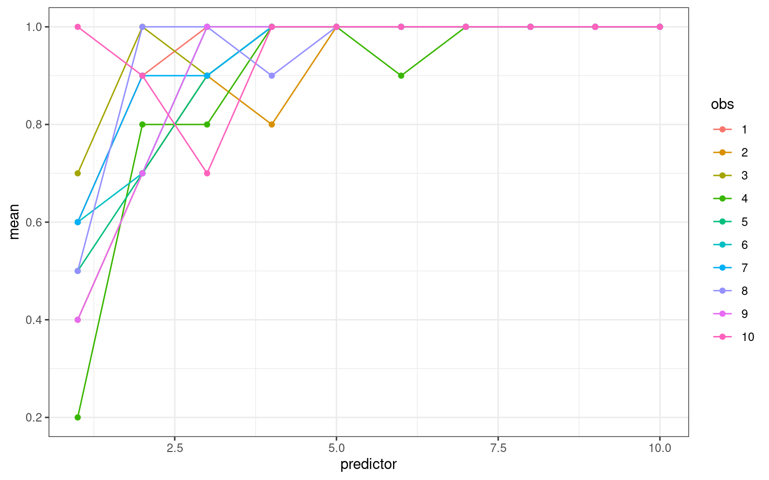
Let’s aggregate the data in two ways: first by just taking the sum of successes/total cases so we can model it using the two-column approach, and second by calculating the mean accuracy
data.agg <- aggregate(outcome, list(predictor = predictor, obs = obs), sum)
data.agg$n <- aggregate(outcome, list(predictor), length)$x
data.agg$sub <- as.factor(data.agg$obs)
data.agg$prob <- aggregate(outcome, list(predictor = predictor, obs = as.factor(obs)),
    mean)$x
We can fit a logistic model either to the two column matrix of x and (n-x) in (number of successes out of total), or on the probability values in agg2. In both cases, we are likely to have underdispersion because of the repeated measurement of each participant.
m3a <- glm(cbind(x, n - x) ~ predictor + obs, data = data.agg, family = binomial(logit))
m3b <- glm(cbind(x, n - x) ~ predictor + obs, data = data.agg, family = quasibinomial(logit))
summary(m3a)
Call:
glm(formula = cbind(x, n - x) ~ predictor + obs, family = binomial(logit),
    data = data.agg)

Deviance Residuals:
     Min        1Q    Median        3Q       Max
-2.52457  -0.20894   0.06035   0.30616   0.77066

Coefficients:
             Estimate Std. Error z value Pr(>|z|)
(Intercept) -2.536205   0.102294 -24.793  < 2e-16 ***
predictor    0.041770   0.012065   3.462 0.000536 ***
obs          0.003108   0.012024   0.259 0.796014
---
Signif. codes:  0 '***' 0.001 '**' 0.01 '*' 0.05 '.' 0.1 ' ' 1

(Dispersion parameter for binomial family taken to be 1)

    Null deviance: 35.885  on 99  degrees of freedom
Residual deviance: 23.784  on 97  degrees of freedom
AIC: 425.93

Number of Fisher Scoring iterations: 4summary(m3b)
Call:
glm(formula = cbind(x, n - x) ~ predictor + obs, family = quasibinomial(logit),
    data = data.agg)

Deviance Residuals:
     Min        1Q    Median        3Q       Max
-2.52457  -0.20894   0.06035   0.30616   0.77066

Coefficients:
             Estimate Std. Error t value Pr(>|t|)
(Intercept) -2.536205   0.047691 -53.180  < 2e-16 ***
predictor    0.041770   0.005625   7.426 4.35e-11 ***
obs          0.003108   0.005606   0.554    0.581
---
Signif. codes:  0 '***' 0.001 '**' 0.01 '*' 0.05 '.' 0.1 ' ' 1

(Dispersion parameter for quasibinomial family taken to be 0.217352)

    Null deviance: 35.885  on 99  degrees of freedom
Residual deviance: 23.784  on 97  degrees of freedom
AIC: NA

Number of Fisher Scoring iterations: 4
Now, we can detect the under-dispersion stemming from within-subject correlation of repeated measures, as the dispersion parameter ends up being .2. The systematic individual differences produce less randomness than we would expect from the binomial model which assumes all people are the same.
If instead, we use just the probabilities within each subject, we can fit the same models:
m4a <- glm(prob ~ predictor + obs, data = data.agg, family = binomial)
m4b <- glm(prob ~ predictor + obs, data = data.agg, family = quasibinomial)
summary(m4a)
Call:
glm(formula = prob ~ predictor + obs, family = binomial, data = data.agg)

Deviance Residuals:
     Min        1Q    Median        3Q       Max
-0.73793   0.00853   0.03449   0.13090   0.97506

Coefficients:
            Estimate Std. Error z value Pr(>|z|)
(Intercept) -1.13001    1.23288  -0.917  0.35937
predictor    1.11871    0.41925   2.668  0.00762 **
obs          0.05079    0.15421   0.329  0.74189
---
Signif. codes:  0 '***' 0.001 '**' 0.01 '*' 0.05 '.' 0.1 ' ' 1

(Dispersion parameter for binomial family taken to be 1)

    Null deviance: 26.5891  on 99  degrees of freedom
Residual deviance:  6.3633  on 97  degrees of freedom
AIC: 27.017

Number of Fisher Scoring iterations: 8summary(m4b)
Call:
glm(formula = prob ~ predictor + obs, family = quasibinomial,
    data = data.agg)

Deviance Residuals:
     Min        1Q    Median        3Q       Max
-0.73793   0.00853   0.03449   0.13090   0.97506

Coefficients:
            Estimate Std. Error t value Pr(>|t|)
(Intercept) -1.13001    0.36872  -3.065  0.00282 **
predictor    1.11871    0.12539   8.922 2.85e-14 ***
obs          0.05079    0.04612   1.101  0.27353
---
Signif. codes:  0 '***' 0.001 '**' 0.01 '*' 0.05 '.' 0.1 ' ' 1

(Dispersion parameter for quasibinomial family taken to be 0.08944706)

    Null deviance: 26.5891  on 99  degrees of freedom
Residual deviance:  6.3633  on 97  degrees of freedom
AIC: NA

Number of Fisher Scoring iterations: 8
Even though the model complains (non-integer successes), it will fit the data. The coefficients are very different because they are fitting different things, and we would have to be careful trying to predict values. We can look at the predicted versus actual values (transforming with the logit function)
data.agg$fit <- m4b$fitted.values
data.agg$obs <- as.factor(data.agg$obs)
data.agg %>%
    ggplot(aes(x = predictor, y = prob, color = obs)) + geom_point() + geom_line(aes(x = predictor,
    y = fit, color = obs)) + theme_bw()
# logit <- function(lo) {1/(1+exp(-lo))}
# plot(data.agg2$x,logit(predict(m4b)),xlab='Mean accuracy',ylab='Predicted
# accuracy')

# dat <- data.frame(obs=as.factor(obs),predictor,outcome) dat$fitted <-
# predict(m4b,dat)
In this case, we can still fit a logistic model, but one main difference is that the original data set had 1000 points of 0/1 data, but the new data has 100 observations. Because we had equal numbers in each level, it probably did not impact much, but if you had different numbers of observations it could impact the actual prediction. Because of the repeated measures design, we have under-dispersion in each case, but in the probability case it was much larger–because the dispersion model is expecting 0/1 values but getting values between 0 and 1.
Dissecting the logistic regression model
Lets take a look at the probability mechanism underlying this function.
logodds <- function(p) {
    log(p/1 - p)
}  ##The probability of a 'yes' for a given set of predictor values.
logit <- function(lo) {
    1/(1 + exp(-lo))
}  ##This is the inverse of the logodds function. The logistic function will
## map any value of the right hand side (z) to a proportion value between 0 and
## 1 (Manning, 2007)
Predicting based on parameters:
We can use Intercept +/- mother’s weight + smoking to make simple predictions about different aspects. Here are two groups that differ by the smoking coefficient, modeling the impact of mother’s weight on low birth weight.
smoking <- data.frame(motherweight = 0:250, nonsmoker = logit(0.4806 + -0.0154 *
0:250), smoker = logit(0.4806 + 0.9388 + -0.0154 * 0:250)) %>%
pivot_longer(cols = 2:3, values_to = "babyweight", names_to = "Smoking")
ggplot(data = smoking, aes(x = motherweight, y = babyweight, group = Smoking, color = Smoking)) +
geom_line() + theme_bw() + scale_color_manual(values = c("orange", "navy"))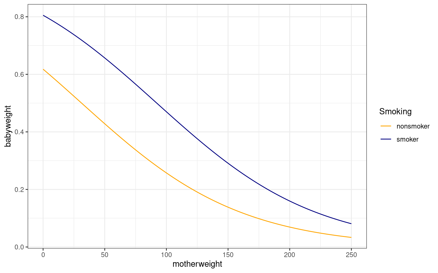 Notice that the impact of smoking is not constant over birth weight, but
it is constant in log-odds terms, meaning the impact of smoking
decreases as the overall probability gets closer to 0 or 1.
Notice that the impact of smoking is not constant over birth weight, but
it is constant in log-odds terms, meaning the impact of smoking
decreases as the overall probability gets closer to 0 or 1.
When we use the ‘predict’ function we can see the probability of a low birth weight baby based on the predictor variables we have chosen. If you look at the birthwt data set it’s interesting to compare the smoking variable with the overall prediction.
We can think about this another way:
coef(partial.model) (Intercept) age lwt factor(race)2 factor(race)3
1.30674122 -0.02552379 -0.01435323 1.00382195 0.44346082 This gives us the change in (log)odds in response to a unit change in the predictor variable if all the other variables are held constant. It can be easier to interpret if the results are exponentiated to put the results in an odds scale.
exp(coef(partial.model)) ## Now we can see that the chances of having a low birth weight baby increase by a factor of (Intercept) age lwt factor(race)2 factor(race)3
3.6941158 0.9747992 0.9857493 2.7286908 1.5580902 ## 5.75 if the mother has a history of hypertension and by 2.92 if the mother
## smokes during pregnancy.
exp(confint(partial.model)) 2.5 % 97.5 %
(Intercept) 0.4752664 32.099365
age 0.9117071 1.039359
lwt 0.9724784 0.997786
factor(race)2 1.0226789 7.322799
factor(race)3 0.7679486 3.167985## gives us the 95 percent confidence interval for each of the coefficients on
## the odds scale. if it includes one we don't know if it has a difference.
## Greater than 1.Example: Personality predicts smartphone choice
Recently, a study was published that establishes that personality factors can predict whether users report using an iphone or android device:
Shaw H, Ellis DA, Kendrick L-R, Ziegler F, Wiseman R. Predicting smartphone operating system from personality and individual differences. Cyberpsychology, Behavior, and Social Networking. 2016 Dec 7;19(12):727-732. Available from, DOI: 10.1089/cyber.2016.0324
Quoting the abstract, “In comparison to Android users, we found that iPhone owners are more likely to be female, younger, and increasingly concerned about their smartphone being viewed as a status object. Key differences in personality were also observed with iPhone users displaying lower levels of Honesty–Humility and higher levels of emotionality.”
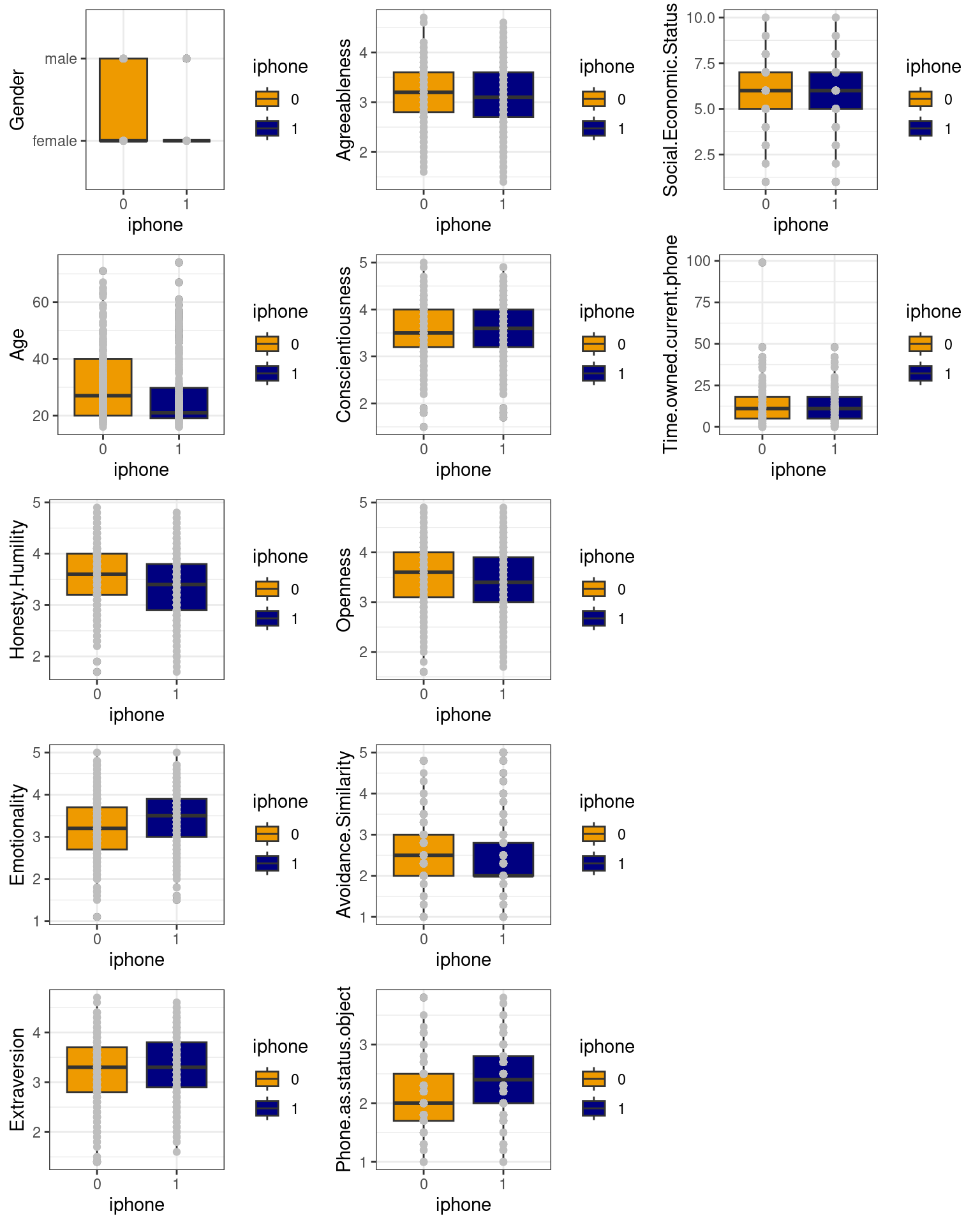
Let’s look at the data and see if we agree.
phone0 <- read.csv("data_study1.csv")
phone0$iphone <- as.factor((phone0$Smartphone == "iPhone") + 0)
phone <- phone0[, -1]
library(grid)

layout <- matrix(1:15, nrow = 5, ncol = 3)
grid.newpage()
pushViewport(viewport(layout = grid.layout(nrow(layout), ncol(layout))))

for (i in 1:12) {
    var <- colnames(phone)[i]
    matchidx <- as.data.frame(which(layout == i, arr.ind = TRUE))
    x <- ggplot(phone, aes_string(x = "iphone", y = var)) + geom_boxplot(aes(group = iphone,
        fill = iphone)) + geom_point(col = "grey") + theme_bw() + scale_fill_manual(values = c("orange2",
        "navy"))
    print(x, vp = viewport(layout.pos.row = matchidx$row, layout.pos.col = matchidx$col))
}
phone2 <- phone
phone2$Gender <- as.numeric(phone2$Gender)
phone2$iphone <- as.numeric(phone2$iphone)
table(phone$iphone)
  0   1
219 310 round(cor(as.matrix(phone2)), 3) Gender Age Honesty.Humility Emotionality
Gender 1 NA NA NA
Age NA 1.000 0.264 -0.222
Honesty.Humility NA 0.264 1.000 0.040
Emotionality NA -0.222 0.040 1.000
Extraversion NA 0.113 0.036 -0.147
Extraversion Agreeableness Conscientiousness Openness
Gender NA NA NA NA
Age 0.113 0.046 0.081 0.166
Honesty.Humility 0.036 0.337 0.289 0.060
Emotionality -0.147 0.014 0.088 -0.146
Extraversion 1.000 0.090 0.054 0.162
Avoidance.Similarity Phone.as.status.object
Gender NA NA
Age 0.092 -0.247
Honesty.Humility 0.027 -0.424
Emotionality -0.140 0.172
Extraversion 0.014 0.054
Social.Economic.Status Time.owned.current.phone iphone
Gender NA NA NA
Age 0.067 0.082 -0.174
Honesty.Humility 0.015 0.063 -0.194
Emotionality -0.079 -0.087 0.159
Extraversion 0.303 0.072 0.069
[ reached getOption("max.print") -- omitted 8 rows ]We see here that approximately 60% of respondents used the iphone–so we could be 60% correct just by claiming everyone chooses the iPhone. The correlations between phone choice and any individual personality trait or related question are all small–with the largest around .24. Because iPhone ownership can be categerized into two categories, a logistic regression model is appropriate:
model.full <- glm(iphone ~ ., data = phone, family = binomial())
summary(model.full)
Call:
glm(formula = iphone ~ ., family = binomial(), data = phone)

Deviance Residuals:
    Min       1Q   Median       3Q      Max
-2.2383  -1.0875   0.6497   0.9718   1.8392

Coefficients:
                           Estimate Std. Error z value Pr(>|z|)
(Intercept)               3.158e-01  1.382e+00   0.228  0.81929
Gendermale               -6.356e-01  2.276e-01  -2.792  0.00523 **
Age                      -1.429e-02  7.689e-03  -1.859  0.06305 .
Honesty.Humility         -5.467e-01  1.918e-01  -2.850  0.00437 **
Emotionality              1.631e-01  1.626e-01   1.003  0.31598
Extraversion              3.161e-01  1.603e-01   1.972  0.04859 *
Agreeableness             4.070e-02  1.672e-01   0.243  0.80770
Conscientiousness         2.802e-01  1.710e-01   1.639  0.10130
Openness                 -1.441e-01  1.635e-01  -0.881  0.37827
Avoidance.Similarity     -2.653e-01  1.175e-01  -2.257  0.02399 *
Phone.as.status.object    5.004e-01  1.931e-01   2.592  0.00955 **
Social.Economic.Status   -1.781e-02  6.741e-02  -0.264  0.79162
Time.owned.current.phone  4.048e-06  9.608e-03   0.000  0.99966
---
Signif. codes:  0 '***' 0.001 '**' 0.01 '*' 0.05 '.' 0.1 ' ' 1

(Dispersion parameter for binomial family taken to be 1)

    Null deviance: 717.62  on 528  degrees of freedom
Residual deviance: 644.17  on 516  degrees of freedom
AIC: 670.17

Number of Fisher Scoring iterations: 4
Looking at the results, we can see that a handful of predictors are significant. Importantly, gender and phone-as-status-object are fairly strong, as well as avoidance of similarity.
Some things to note:
- Negative and positive coefficients still compute relative odds in favor/against choosing an iPhone.
- Residual deviance is about the same as residual DF, so we should not worry about over-dispersion.
- Inter-correlations between big-five personality dimensions are sometimes sizeable, but only extraversion predicts phone use.
Trying to make more sense of the estimates,. Notice if we transform the intercept to probability space with logit transform, we get a value that is almost exactly the base rate of about 58%. This makes sense because if we had no other information, we’d give any user a 58% chance of having an iphone, and going with our best guess, we would be correct 58% of the time. All the other coefficients will modify this percentage. To get a better understanding of how the modification works, let’s just do a exp() transform on the coefficients to compute the odds. A value of 1.0 indicates even-odds–basically no impact. Note that these values are not symmetric around 1.0: .5 would be the multiplicative opposite of 2.0.
logit <- function(lo) {
    1/(1 + exp(-lo))
}
logit(model.full$coefficients[1])  ##intercept
(Intercept)
0.5782903 mean(phone$iphone)[1] NAexp(model.full$coefficients) ##odds ratio for each coefficient (Intercept) Gendermale Age
1.3712996 0.5296061 0.9858082
Honesty.Humility Emotionality Extraversion
0.5788340 1.1771187 1.3717738
Agreeableness Conscientiousness Openness
1.0415385 1.3233525 0.8658186
Avoidance.Similarity Phone.as.status.object Social.Economic.Status
0.7669790 1.6494402 0.9823474
Time.owned.current.phone
1.0000040 Perhaps as expected, no individual question helps a lot, except for gender and ‘phone as a status symbol’. The abstract points out that users tend to be younger, which is true if you look at the correlations as well. The coefficients of .985 means that for every year older you get, you decrease the odds in owning an iphone by this multiplier. The other measures are typically on a multi-point scale (probably 4 to 7-point scale), so the same interpretation can be made. For conscientiousness, each unit increase in conscientiousness increases the odds by 1.32 that you own an iPhone.
Of course, we’d maybe want to reduce the complexity of the model, especially if we were trying to predict something. We can automatically pick a smaller model using the AIC statistic and the step function:
small <- step(model.full, direction = "both", trace = F)
print(small)
Call:  glm(formula = iphone ~ Gender + Age + Honesty.Humility + Extraversion +
    Conscientiousness + Avoidance.Similarity + Phone.as.status.object,
    family = binomial(), data = phone)

Coefficients:
           (Intercept)              Gendermale                     Age
               0.43333                -0.75829                -0.01642
      Honesty.Humility            Extraversion       Conscientiousness
              -0.49910                 0.25761                 0.27186
  Avoidance.Similarity  Phone.as.status.object
              -0.27811                 0.56146

Degrees of Freedom: 528 Total (i.e. Null);  521 Residual
Null Deviance:      717.6
Residual Deviance: 646.1 AIC: 662.1summary(small)
Call:
glm(formula = iphone ~ Gender + Age + Honesty.Humility + Extraversion +
    Conscientiousness + Avoidance.Similarity + Phone.as.status.object,
    family = binomial(), data = phone)

Deviance Residuals:
    Min       1Q   Median       3Q      Max
-2.2574  -1.1113   0.6450   0.9674   1.8806

Coefficients:
                        Estimate Std. Error z value Pr(>|z|)
(Intercept)             0.433333   1.094625   0.396 0.692198
Gendermale             -0.758290   0.201727  -3.759 0.000171 ***
Age                    -0.016422   0.007519  -2.184 0.028947 *
Honesty.Humility       -0.499100   0.180133  -2.771 0.005593 **
Extraversion            0.257610   0.147444   1.747 0.080608 .
Conscientiousness       0.271859   0.165416   1.643 0.100283
Avoidance.Similarity   -0.278105   0.115451  -2.409 0.016002 *
Phone.as.status.object  0.561465   0.183301   3.063 0.002191 **
---
Signif. codes:  0 '***' 0.001 '**' 0.01 '*' 0.05 '.' 0.1 ' ' 1

(Dispersion parameter for binomial family taken to be 1)

    Null deviance: 717.62  on 528  degrees of freedom
Residual deviance: 646.09  on 521  degrees of freedom
AIC: 662.09

Number of Fisher Scoring iterations: 4
This seems like a reasonably small model. The residual deviance is relatively small, so we won’t worry about over-dispersion. How well does it do? One way to look is to compute a table predicting iphone ownership based on the model’s prediction.
cat("total iPhones: ", sum(as.numeric(phone$iphone)), "\n")total iPhones: 839 cat("Full model\n")Full modeltab <- table(model.full$fitted.values > 0.5, phone$iphone) ##365 correct
print(tab)
          0   1
  FALSE 114  59
TRUE 105 251print(sum(diag(tab)))[1] 365print(sum(diag(tab))/sum(tab))[1] 0.6899811cat("\n\nSmall model\n")
Small modeltab <- table(small$fitted.values > 0.5, phone$iphone) ##361 correct
print(tab)
          0   1
  FALSE 113  62
TRUE 106 248print(sum(diag(tab)))[1] 361print(sum(diag(tab))/sum(tab))[1] 0.6824197Notice that we could get 310 correct (58%) just by guessing ‘iphone’ for everyone. For the complex model, this improves to 365 correct–by about 50 additional people, or 10% of the study population. The reduced model only drops our prediction by 4 people, so it seems reasonable. We’d may want to use a better criterion for variable selection if we were really trying to predict (such as cross-validation), but this seems OK for now.
But first let’s challenge the results a little more. Suppose we just looked at the two demographic predictors–gender and age:
tiny <- glm(iphone ~ Gender + Age, data = phone, family = binomial())
summary(tiny)
Call:
glm(formula = iphone ~ Gender + Age, family = binomial(), data = phone)

Deviance Residuals:
    Min       1Q   Median       3Q      Max
-1.5951  -1.2026   0.8382   0.9236   1.5615

Coefficients:
             Estimate Std. Error z value Pr(>|z|)
(Intercept)  1.359424   0.231616   5.869 4.38e-09 ***
Gendermale  -0.772004   0.192041  -4.020 5.82e-05 ***
Age         -0.026006   0.006989  -3.721 0.000199 ***
---
Signif. codes:  0 '***' 0.001 '**' 0.01 '*' 0.05 '.' 0.1 ' ' 1

(Dispersion parameter for binomial family taken to be 1)

    Null deviance: 717.62  on 528  degrees of freedom
Residual deviance: 685.37  on 526  degrees of freedom
AIC: 691.37

Number of Fisher Scoring iterations: 4
tab <- table(tiny$fitted.values > 0.5, phone$iphone) ##339 correct
print(tab)
          0   1
  FALSE  80  56
TRUE 139 254print(sum(diag(tab)))[1] 334sum(diag(tab))/sum(tab)[1] 0.63138This gets us 334 correct (63%), up from 310 (58.6%) we can get by chance, but below the ~360 number we otherwise achieved. The lesson is that knowing nothing will make us 59% correct; knowing age/gender will get us 63% correct, and knowing a bunch of personality information will get us 68% correct.
This is a bit less exciting than some of the news coverage made it seem. If the authors had said “we improved to 10% over chance and 5% over demographics by using personality variables”, or “we correctly classified about 25/500 additional people using personality information”, the results seems less compelling. One question would be could you use this information as a phone vendor to make money? You could certainly mis-use it and end up wasting money via targetted advertising and the like.
##Probit regression Sometimes people choose probit regression, which uses a normal density function as the link, instead of the logistic. This is akin to doing a normal linear regression on logit-transformed data. If we use this here, we see that the values actually don’t change much–the particular coefficients change, but their p-values and AIC values are essentially unchanged. These two transforms have an almost identical shape. The logistic is typically a bit easier to work with (it can be integrated exactly instead of just numerically), and in many fields it is typical to interpret odds ratios and so logistic regression would be preferred. However, there are some domains where probit regression is more typical.
tiny2 <- glm(iphone ~ Gender + Age, data = phone, family = binomial(link = "probit"))
summary(tiny2)
Call:
glm(formula = iphone ~ Gender + Age, family = binomial(link = "probit"),
    data = phone)

Deviance Residuals:
    Min       1Q   Median       3Q      Max
-1.5977  -1.2026   0.8370   0.9241   1.5621

Coefficients:
             Estimate Std. Error z value Pr(>|z|)
(Intercept)  0.843829   0.141171   5.977 2.27e-09 ***
Gendermale  -0.478495   0.118885  -4.025 5.70e-05 ***
Age         -0.016135   0.004313  -3.741 0.000183 ***
---
Signif. codes:  0 '***' 0.001 '**' 0.01 '*' 0.05 '.' 0.1 ' ' 1

(Dispersion parameter for binomial family taken to be 1)

    Null deviance: 717.62  on 528  degrees of freedom
Residual deviance: 685.31  on 526  degrees of freedom
AIC: 691.31

Number of Fisher Scoring iterations: 4
tab <- table(tiny2$fitted.values > 0.5, phone$iphone)
print(tab)
          0   1
  FALSE  80  56
TRUE 139 254print(sum(diag(tab)))[1] 334print(sum(diag(tab))/sum(tab))[1] 0.63138