Multinomial Regression
Modeling categorical outcomes with more than two levels
The generalized linear regression adapt linear regression with a transformation (link) and distribution (alternative to gaussian) with maximum-likelihood estimation. With logistic regression, we saw how we could essentially transform linear regression into predicting the likelihood of being in one of two binary states, using a binomial model. What if you have more than two categories? This would be a multinomial (rather than binomial) model.
Separate one-dimensional logistics
At a high level, a reasonable approach might be to fit a separate logistic model for each category, where we predict the target is or is not part of the category. We can do this by hand for the iris data set:
lm1 <- glm((Species == "setosa") ~ Sepal.Length + Sepal.Width + Petal.Length + Petal.Width,
    family = binomial, data = iris)
lm2 <- glm((Species == "versicolor") ~ Sepal.Length + Sepal.Width + Petal.Length +
    Petal.Width, family = binomial, data = iris)
lm3 <- glm((Species == "virginica") ~ Sepal.Length + Sepal.Width + Petal.Length +
    Petal.Width, family = binomial, data = iris)

summary(lm1)
Call:
glm(formula = (Species == "setosa") ~ Sepal.Length + Sepal.Width +
    Petal.Length + Petal.Width, family = binomial, data = iris)

Deviance Residuals:
       Min          1Q      Median          3Q         Max
-3.185e-05  -2.100e-08  -2.100e-08   2.100e-08   3.173e-05

Coefficients:
               Estimate Std. Error z value Pr(>|z|)
(Intercept)     -16.946 457457.096       0        1
Sepal.Length     11.759 130504.039       0        1
Sepal.Width       7.842  59415.383       0        1
Petal.Length    -20.088 107724.592       0        1
Petal.Width     -21.608 154350.613       0        1

(Dispersion parameter for binomial family taken to be 1)

    Null deviance: 1.9095e+02  on 149  degrees of freedom
Residual deviance: 3.2940e-09  on 145  degrees of freedom
AIC: 10

Number of Fisher Scoring iterations: 25summary(lm2)
Call:
glm(formula = (Species == "versicolor") ~ Sepal.Length + Sepal.Width +
    Petal.Length + Petal.Width, family = binomial, data = iris)

Deviance Residuals:
    Min       1Q   Median       3Q      Max
-2.1280  -0.7668  -0.3818   0.7866   2.1202

Coefficients:
             Estimate Std. Error z value Pr(>|z|)
(Intercept)    7.3785     2.4993   2.952 0.003155 **
Sepal.Length  -0.2454     0.6496  -0.378 0.705634
Sepal.Width   -2.7966     0.7835  -3.569 0.000358 ***
Petal.Length   1.3136     0.6838   1.921 0.054713 .
Petal.Width   -2.7783     1.1731  -2.368 0.017868 *
---
Signif. codes:  0 '***' 0.001 '**' 0.01 '*' 0.05 '.' 0.1 ' ' 1

(Dispersion parameter for binomial family taken to be 1)

    Null deviance: 190.95  on 149  degrees of freedom
Residual deviance: 145.07  on 145  degrees of freedom
AIC: 155.07

Number of Fisher Scoring iterations: 5summary(lm3)
Call:
glm(formula = (Species == "virginica") ~ Sepal.Length + Sepal.Width +
    Petal.Length + Petal.Width, family = binomial, data = iris)

Deviance Residuals:
     Min        1Q    Median        3Q       Max
-2.01105  -0.00065   0.00000   0.00048   1.78065

Coefficients:
             Estimate Std. Error z value Pr(>|z|)
(Intercept)   -42.638     25.708  -1.659   0.0972 .
Sepal.Length   -2.465      2.394  -1.030   0.3032
Sepal.Width    -6.681      4.480  -1.491   0.1359
Petal.Length    9.429      4.737   1.990   0.0465 *
Petal.Width    18.286      9.743   1.877   0.0605 .
---
Signif. codes:  0 '***' 0.001 '**' 0.01 '*' 0.05 '.' 0.1 ' ' 1

(Dispersion parameter for binomial family taken to be 1)

    Null deviance: 190.954  on 149  degrees of freedom
Residual deviance:  11.899  on 145  degrees of freedom
AIC: 21.899

Number of Fisher Scoring iterations: 12
If we want to predict the probability of each class, we end up with some problems. If we look at the ’‘’probability’’’ of each membership from each separate model (taking logit), the three do not sum to 1.0! We can normalize and come up with an answer, but this seems rather ad hoc. In this case, we only made 3 errors, but maybe there is a better way.
logit <- function(x) {
    1/(1 + exp(-x))
}
modelpreds <- cbind(predict(lm1), predict(lm2), predict(lm3))
hist(rowSums(logit(modelpreds)))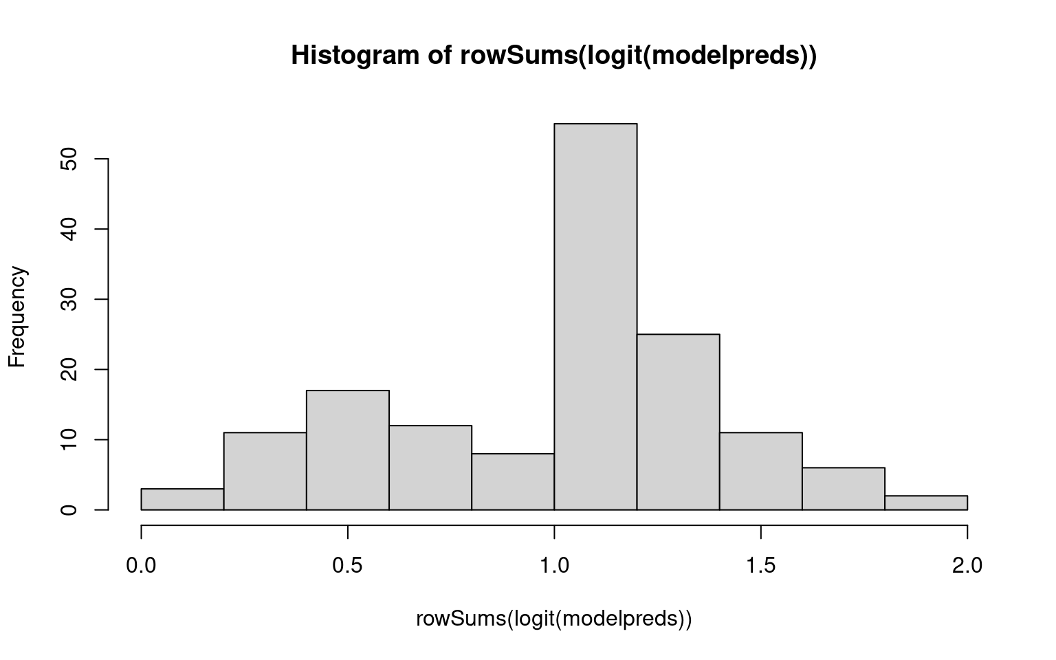
# normalize them here:
probs <- (exp(modelpreds)/rowSums(exp(modelpreds)))
head(round(probs, 3))
[,1] [,2] [,3]
1 1 0 0
2 1 0 0
3 1 0 0
4 1 0 0
5 1 0 0
6 1 0 0class <- apply(probs, 1, which.max)
table(iris$Species, class) class
1 2 3
setosa 50 0 0
versicolor 0 48 2
virginica 0 1 49Computing binary decision criteria
By computing exp(beta)/sum(exp(beta), we can get an estimated probability of each group membership–ensuring they sum to 1.0. Alternately, we could compare the probabilities of any pairing by taking the sum of two columns
plot(logit(modelpreds[, 1] - modelpreds[, 2]), main = "Setosa vs. Versicolor")
plot(logit(modelpreds[, 1] - modelpreds[, 3]), main = "Setosa vs. Virginica")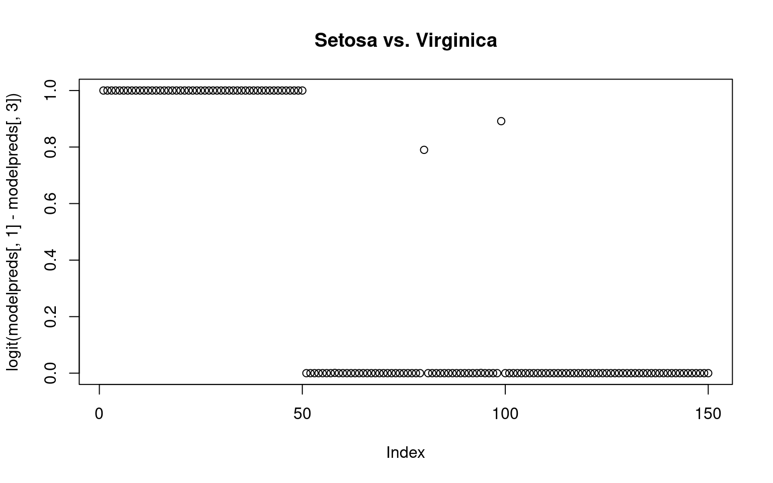
plot(logit(modelpreds[, 2] - modelpreds[, 3]), main = "Versicolor vs. Virginica")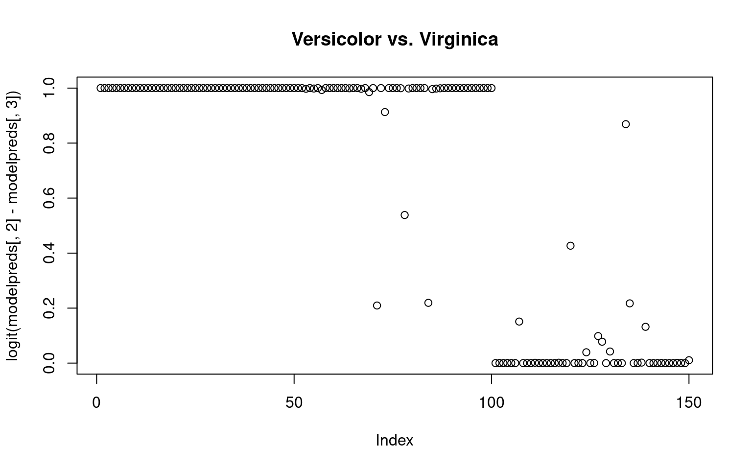 ## The multinom model However, this doesn’t fit all the information
simultaneously, and so the separation is pretty minimal. We can fit this
within a poisson glm (See the Faraway book for examples, treating
species as a predictor, and the count as the dependent variable), but
the nnet library has a multinom function that will do exactly this, but
sort of treat the species as the predicted variable. Instead of three
models, it essentially fits two log-transform models, each in comparison
to the first level of the DV. This is a log-ratio model, which is
consequently akin to the log-odds transform.
## The multinom model However, this doesn’t fit all the information
simultaneously, and so the separation is pretty minimal. We can fit this
within a poisson glm (See the Faraway book for examples, treating
species as a predictor, and the count as the dependent variable), but
the nnet library has a multinom function that will do exactly this, but
sort of treat the species as the predicted variable. Instead of three
models, it essentially fits two log-transform models, each in comparison
to the first level of the DV. This is a log-ratio model, which is
consequently akin to the log-odds transform.
library(nnet)


model <- multinom(Species ~ Sepal.Length + Sepal.Width + Petal.Length + Petal.Width,
    data = iris)
# weights: 18 (10 variable)
initial value 164.791843
iter 10 value 16.177348
iter 20 value 7.111438
iter 30 value 6.182999
iter 40 value 5.984028
iter 50 value 5.961278
iter 60 value 5.954900
iter 70 value 5.951851
iter 80 value 5.950343
iter 90 value 5.949904
iter 100 value 5.949867
final value 5.949867
stopped after 100 iterationssummary(model)Call:
multinom(formula = Species ~ Sepal.Length + Sepal.Width + Petal.Length +
Petal.Width, data = iris)
Coefficients:
(Intercept) Sepal.Length Sepal.Width Petal.Length Petal.Width
versicolor 18.69037 -5.458424 -8.707401 14.24477 -3.097684
virginica -23.83628 -7.923634 -15.370769 23.65978 15.135301
Std. Errors:
(Intercept) Sepal.Length Sepal.Width Petal.Length Petal.Width
versicolor 34.97116 89.89215 157.0415 60.19170 45.48852
virginica 35.76649 89.91153 157.1196 60.46753 45.93406
Residual Deviance: 11.89973
AIC: 31.89973 predict(model) [1] setosa setosa setosa setosa setosa setosa
[7] setosa setosa setosa setosa setosa setosa
[13] setosa setosa setosa setosa setosa setosa
[19] setosa setosa setosa setosa setosa setosa
[25] setosa setosa setosa setosa setosa setosa
[31] setosa setosa setosa setosa setosa setosa
[37] setosa setosa setosa setosa setosa setosa
[43] setosa setosa setosa setosa setosa setosa
[49] setosa setosa versicolor versicolor versicolor versicolor
[55] versicolor versicolor versicolor versicolor versicolor versicolor
[61] versicolor versicolor versicolor versicolor versicolor versicolor
[67] versicolor versicolor versicolor versicolor versicolor versicolor
[73] versicolor versicolor versicolor
[ reached getOption("max.print") -- omitted 75 entries ]
Levels: setosa versicolor virginicahead(round(predict(model, type = "probs"), 4)) setosa versicolor virginica
1 1 0 0
2 1 0 0
3 1 0 0
4 1 0 0
5 1 0 0
6 1 0 0table(iris$Species, predict(model))
             setosa versicolor virginica
  setosa         50          0         0
  versicolor      0         49         1
  virginica       0          1        49
For this data set, we get almost perfect classification–better than with the separate models. The coefficients for each model indicate the log-probability ratio of each model to the baseline. To compare two other models, we can just take the difference of these values, because the denominator of the first model will cancel out.
Overall, this is useful for predicting, but could you do hypothesis testing as well? Let’s remove one of the predictors:
model2 <- multinom(Species ~ Sepal.Length + Sepal.Width + Petal.Length, data = iris)# weights: 15 (8 variable)
initial value 164.791843
iter 10 value 21.394999
iter 20 value 13.010468
iter 30 value 11.932227
iter 40 value 11.899523
iter 50 value 11.886536
final value 11.886441
convergedanova(model, model2) Model Resid. df Resid. Dev
1 Sepal.Length + Sepal.Width + Petal.Length 292 23.77288
2 Sepal.Length + Sepal.Width + Petal.Length + Petal.Width 290 11.89973
Test Df LR stat. Pr(Chi)
1 NA NA NA
2 1 vs 2 2 11.87315 0.002641063Now, comparing the two model,s, we can see there is a significant difference, indicating that Sepal.Length is an important predictor.