Parameters and Knot Vectors for Surfaces

Since a B-spline surface of degree (p,q) defined by e+1 rows and f+1 columns of control points has the following equation

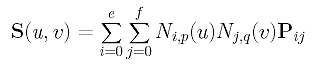
it requires two sets of parameters for surface interpolation and approximation. Suppose we have m+1 rows and n+1 columns of data points D_ij, where 0 <= i <= m and 0 <= j <= n. Thus, m+1 parameters s₀, ..., s_m in the u-direction (i.e., one for each row of data points) and n+1 parameters t₀, ..., t_n in the v-direction (i.e., one for each column of data points) are required so that point (s_c,t_d) in the domain of the surface corresponds to point S(s_c,t_d) on the surface, which, in turn, corresponds to the data point D_cd. Putting this in an equation form, the point on the surface, evaluated at (s_c,t_d) as shown below,

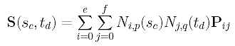
corresponds to the data point D_cd, where s_c and t_d are parameters in the u- and v-direction, respectively.

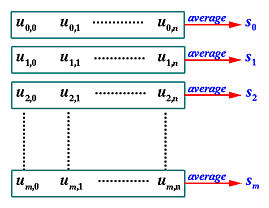
In the equation of the desired B-spline surface, the u-direction corresponds to the index i in N_i,p(u) and P_ij. Since i runs from 0 to m, N_0,p(u), N_1,p(u), ..., N_m,p(u) are coefficients of the columns of the control points. Therefore, in the u-direction, we need m+1 parameters, and using a parameter computation method that takes degree p and the data points on column j, we can compute m+1 parameters u_0,j, u_1,j, ..., u_m,j. This is shown in the figure below. The desired parameters s₀, s₁, ..., s_m are simply the average of each row. More precisely, parameter s_i is the average of parameters on row i, s_i = (u_i,0 + u_i,1 + ... + u_i,n)/(n+1).

The computation of parameters for the v-direction is similar. Each row of data points has n+1 points and hence requires n+1 parameters. Thus, for data points on row i, we can compute n+1 parameter values v_i,0, v_i,1, ..., v_i,n. Since we have m+1 rows, these values can be organized into a (m+1)×(n+1) matrix, and parameter t_j is simply the average of the parameters on column j, t_j = (v_0,j + v_1,j + ... + v_m,j)/(m+1). In this way, we obtain n+1 parameters for the v-direction.

This procedure is summarized as follows:

Input: (m+1)×(n+1) data points D_i,j;
Output: Parameters in the u-direction s₀, ..., s_m
and parameters in the v-direction t₀, ..., t_n;
Algorithm:

₀

for

_0,j

_1,j

_m,j

for

_i,0

_i,1

_i,n

₀

for

_i,0

_i,1

_i,n

for

_0,j

_1,j

_n,j

Then, parameter values s₀, s₁, ..., s_m and degree p jointly define a knot vector U in the u-direction. Similarly, parameters t₀, t₁, ..., t_n and degree q jointly define a knot vector V in the v-direction. Click here to review the way of computing a knot vector from a set of parameters.

Note that the above is only a conceptual algorithm and is inefficient. Once you know what is going on, it is quite easy to convert it to a very efficient algorithm. Note also that this algorithm only works for the uniformly spaced, chord length and centripetal methods. For the universal method, because there is no data points involved, we can apply uniform knots to one row and one column of data points for computing the parameters.