


The meaning of knot insertion is adding a new knot into the existing knot vector without changing the shape of the curve. This new knot may be equal to an existing knot and, in this case, the multiplicity of that knot is increased by one. Because of the fundamental equality m = n + p + 1, after adding a new knot, the value of m is increased by one and, consequently, either the number of control points or the degree of the curve must also be increased by one. Changing the degree of the curve due to the increase of knots will change the shape of the curve globally and will not be considered. Therefore, inserting a new knot causes a new control point to be added. In fact, some existing control points are removed and replaced with new ones by corner cutting.
Although knot insertion looks like not very interesting, it is one of the most important algorithms for B-spline curves since many other useful algorithms are based on knot insertion. Therefore, we shall start important algorithms with knot insertion. In the following, we shall present an algorithm for inserting a single knot, followed by an algorithm for inserting a single knot multiple times.
The left figure below shows a clamped B-spline curve of degree 4 with uniform knots, while the right figure shows the result after a new knot u = 0.5 is inserted. The left figure also shows the control polylines before and after the insertion. As you can see, the shape of the curve does not change. However, the defining control polyline is changed. In fact, four new control points in red replace the original control points P4, P5 and P6, and three line segments in yellow cut the corners at P4, P5 and P6.

Suppose the new knot t lies in knot span [uk, uk+1). From the strong convex hull property, C(t) lies in the convex hull defined by control points Pk, Pk-1, ..., Pk-p and the basis functions of all other control points are zero. Thus, the knot insertion computation can be restricted on control points Pk, Pk-1, ..., Pk-p. The way of inserting t is to find p new control points Qk on leg Pk-1Pk, Qk-1 on leg Pk-2Pk-1, ..., and Qk-p+1 on leg Pk-pPk-p+1 such that the old polyline between Pk-p and Pk (in black below) is replaced by Pk-pQk-p+1...QkPk (in orange below) by cutting the corners at Pk-p+1, ..., Pk-1. All other control points are unchanged. Note that p-1 control points of the original control polyline are removed and replaced with p new control points.

Fortunately, the positions of new control points Qi's are easy to compute. The formula for computing the new control point Qi on leg Pi-1Pi is the following:

where the ratio ai is computed as below:

In summary, to insert a new knot t, we first find the knot span [uk, uk+1) that contains t. With k available, p new control points Qk-p+1, ..., Qk are computed with the above formula. Finally, the original control polyline between Pk-p and Pk is replaced with the new polyline defined by Pk-p, Qk-p+1, Qk-p+2, ..., Qk-1, Qk and Pk. Note that after inserting a new knot, the knot vector becomes u0, u1, ..., uk, t, uk+1, ..., and um. If the new knot t is equal to uk, the multiplicity of uk is increased by one.
The above computation scheme can be illustrated with the following diagram. First, the affected control points are listed on the left column. Then, the computed new control points are listed on the second column. Note that the number of new control points is one less than the affected control points. The computation of new control point Qi, where k-p+1 <= i <= k, requires two original control points Pi-1 and Pi with coefficients 1-ai and ai, respectively. After the computation, use the points surrounded by the blue dotted line to replace those not in the region. All unaffected control points are preserved. Therefore, the original set of control points Pk-p, Pk-p+1, ..., Pk-1, Pk is replaced with Pk-p, Qk-p+1, ..., Qk-1, Pk.

Let us take a look at a geometric interpretation of ai. From its definition, ai:1-ai is the ratio of dividing interval [ui, ui+p) by the value of t as shown below:

There are k ai's, each of which covers p knot spans (i.e., [ui, ui+p)). If we stack these intervals together and align them at the value of t, we have the following diagram:

Therefore, the position of t divides knot spans
[uk, uk+p),
[uk-1, uk+p-1), ...,
[uk-p+1, uk+1) into ratios
ak, ak-1, ...,,
ak-p+1, which, in turn, provide the ratios
for dividing legs
PkPk-1,
Pk-1Pk-2, ...
Pk-pPk-p+1.
Example 1: Inserting a Knot in a Knot Span
Suppose we have a B-spline curve of degree 3 with a knot vector as follows:
| u0 to u3 | u4 | u5 | u6 | u7 | u8 to u11 |
| 0 | 0.2 | 0.4 | 0.6 | 0.8 | 1 |
We want to insert a new knot t = 0.5. Since t = 0.5 lies in knot span [u5,u6), the affected control points are P5, P4, P3 and P2. To determine the three new control points Q5, Q4 and Q3, we need to compute a5, a4 and a3 as follows:

The three new control points are

The new control polyline becomes P0, P1, P2, Q3, Q4, Q5, P5, ...., and the new knot vector is
| u0 to u3 | u4 | u5 | u6 | u7 | u8 | u9 to u12 |
| 0 | 0.2 | 0.4 | 0.5 | 0.6 | 0.8 | 1 |
Since the original B-spline curve has p = 3 and m = 11, we have n = m - p - 1 = 11 - 3 - 1 = 7 and hence 8 control points. The following is a B-spline curve satisfying this condition and its basis functions:

The three blue rectangles are Q3, Q4 and Q5. After inserting t = 0.5, the corners at P3 and P4 are cut, yielding the following B-spline curve and its basis functions. Note that the shape of the curve does not change:


The following diagram shows the relationship between the old and new control points. Note that the new set of control points contains P0, P1, P2, Q3, Q4, Q5, P5, P6 and P7.

The relationship among aj's, uj's, and t are shown below:

Example 2: Inserting a Knot at an Existing Simple Knot
Suppose we have a knot vector as follows:
| u0 to u4 | u5 | u6 | u7 | u8 | u9 | u10 | u11 | u12 to u16 |
| 0 | 0.125 | 0.25 | 0.375 | 0.5 | 0.625 | 0.75 | 0.875 | 1 |
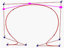
We want to insert a new knot t = 0.5, which is equal to an existing one (i.e., t = u8 = 0.5). The following is a B-spline curve of degree 4 and its basis functions before the new knot t is inserted.


Since t is in [u8,u9), the affected control points are P8, P7, P6, P5 and P4. The coefficients are computed as follows:

The new control points are

The new control point Q8 is equal to the original control point P7. In fact, if t is equal to a knot, say uk, then

Consequently, we have

That is, if the new knot t to be inserted is equal to an existing simple knot uk, then Qk, the last new control point, is equal to Pk-1. The following diagram shows the computation scheme:

The figure shown at the beginning of this example shows the new control points and the new control polyline in orange, Note that the new control points are P0, P1, P2, P3, P4, Q5, Q6, Q7, Q8 = P7, P8, P9, P10 and P11. The curve and its basis functions after the new knot t = 0.5 is inserted is shown below.


The relationship among aj's, uj's, and t are shown below:

Example 3: Inserting a Knot at an Existing Multiple Knot
What if the new knot t is inserted at a multiple knot? Suppose t is inserted at knot uk of multiplicity s. Hence, we have s consecutive equal knots: uk = uk-1 = uk-2 = .... = uk-s+1 and uk-s+1 being not equal to uk-s. In the computation of coefficients ak, ...., ak-p+1, we have the following:

Hence, coefficients ak, ...., ak-p+1 are all zero and, consequently, we have

This shows that if the new knot t is inserted at a knot uk of multiplicity s, then the last s new control points, Qk, Qk-1, ..., Qk-s+1 are equal to the original control points Pk-1, Pk-2, ..., Pk-s. If s = 1 (i.e., simple knot), Qk is equal to Pk-1, which is exactly what is discussed in Example 2. If s = 0 (i.e., t is not a knot), then all control points from Pk-p to Pk are involved. This is the case of Example 1. The following diagram shows the computation scheme:
