Bézier Surfaces: de Casteljau's Algorithm

De Casteljau's algorithm can be extended to handle Bézier surfaces. More precisely, de Casteljau's algorithm can be applied several times to find the corresponding point on a Bézier surface p(u,v) given (u,v). This page describes such as extension, which is based on the concept of isoparametric curves discussed in the previous page.

Recall that the equation of a Bézier surface

can be rewritten as the following

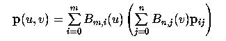
For i = 0, 1, ..., m define q_i(v) as follows:

For a fixed v, we have m+1 points q₀(v), q₁(v), ..., q_m(v). Each q_i(v) is a point on the Bézier curve defined by control points p_i0, p_i1, ..., p_in. Plugging these back into the surface equation yields

This means p(u,v) is a point of the Bézier curve defined by m+1 control points q₀(v), q₁(v), ..., q_m(v). Thus, we have the following conclusion:

To find point p(u,v) on a Bézier surface, we can find m+1 points q₀(v), q₁(v), ..., q_m(v) and then from these points find p(u,v).

This conclusion gives us a simple way for computing p(u,v) given (u,v). Here is why. Since each q_i(v) is a point on the Bézier curve defined by the i-th row of control points: p_i0, p_i1, ..., p_in. Therefore, for the i-th row and a given v, we can apply de Casteljau's algorithm for Bézier curve to compute q_i(v). After m+1 applications of de Casteljau's algorithm (i.e., one for each row), we shall have q₀(v), q₁(v), ..., q_m(v) in hand. Then, applying de Casteljau's algorithm to these m+1 control points again with u yields the final point p(u,v) on the surface!

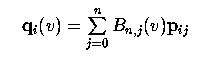
The following diagram illustrates this concept. The given surface is a degree (2,2) Bézier surface defined by a 3x3 control net. Suppose u = 2/3 and v = 1/3. To determine q₀(1/3), we take the 0-th row of control points p₀₀, p₀₁ and p₀₂ and apply de Casteljau's algorithm to this Bézier curve with v = 1/3. Repeat this for the first row and the second row with v = 1/3. This yields three intermediate control points q₀(1/3), q₁(1/3) and q₂(1/3). Finally, apply de Casteljau's algorithm to these three new control points with u = 2/3. The result is p(2/3,1/3) which is colored in yellow in the figure.

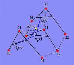
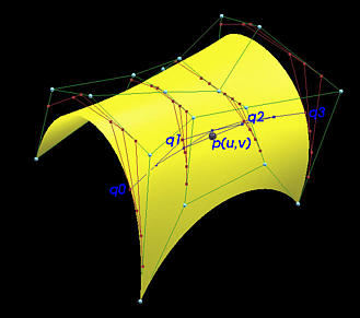
The following is an example with the given Bézier surface displayed. The control points are shown in white. This control net has four rows and five columns and hence is a degree (3,4) Bézier surface. For each row, the intermediate polylines used for the computation of de Casteljau's algorithm is shown in red. The four intermediate control points q₀, q₁, q₂ and q₃ are shown in the figure. The intermediate polylines used for the computation of this application of de Casteljau's algorithm are shown in blue and the final point p(u,v) on the surface is shown as a red sphere.

Finally, the following summarizes this algorithm:

Input: a m+1 rows and n+1 columns of control points and (u,v).
Output: point on surface p(u,v)
Algorithm:


for i := 0 to m do

begin

Apply de Casteljau's algorithm to the i-th row of control points with v;
Let the point obtained be q_i(v);

end
Apply de Casteljau's algorithm to q₀(v), q₁(v), ..., q_m(v) with u;
The point obtained is p(u,v);