This page contains a few components of DesignMentor version 2. Currently, only the Windows version is available.
| Program | Functionality |
| Supporting DLLs | One needs these DLLs to run all components of DesignMentor. Click on the name to download a copy: GLU32.DLL, GLUT32.DLL, and GDI32.DLL. |
| DesignMentor curve system | This is the curve subsystem of DesignMentor. Click here to download its executable. |
| DesignMentor surface system | This is the surface subsystem of DesignMentor. Click here to download its executable. |
| NURBS Visualization | This is an extra component of the curve subsystem of DesignMentor to show the relationship between a 2D NURBS curve and a 3D B-spline curve. This is a late alpha system. Click here to download its executable. |
| Voronoi Region and Delauney Triangulation Visualization | This system is built to show the relation among 3D convex hull, 2D Voronoi region and Delauney triangulation. This is a late alpha system. Click here to download its executable. |
Our systems use GLUT to build the interface. GLU32.DLL, GLUT32.DLL and GDI32.DLL are precompiled GLUT DLLs. You may download these files from GLUT web site. You will also need an OpenGL DLL, which should be part of your Windows system distribution.
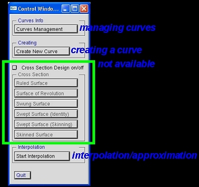
This is a greatly enhanced system of the previous popular version 1. It has a new user interface and many enhanced and new components. The following shows the Control Window #1. This window is used to create a curve, manage the created curves, enters cross-sectional design (not yet available), and starts curve interpolation and approximation.
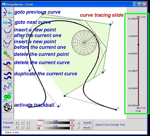
The drawing canvas now has a list of icons for quick actions. The following screen shot shows the meaning of most icons, a B-spline curve, the de Boor net for computing a point on the curve, the strong convex hull property, moving triad, and curvature sphere. A curvature plot of the curve is available in the Curvature Window.
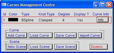
A click on the Curve Management button brings up the Curve Management Center. With this small window, one can add, load, save and import a curve, and create a new scene, load an old scene and save the scene on the drawing canvas. For each curve, its ID, color, type, knot type, degree, display status and its complete information are shown. A click on the type, knot type, degree and display status field of a curve brings up a short menu. By selecting a new setting, one can change the corresponding component of a curve (i.e., changing a B-spline curve to a NURBS) quickly. However, the shape of the curve will be altered. Color change mut be performed with the Change Color Scheme window.
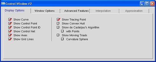
The Control Window #2 has five tabs that show the capability of this new version: Display Options, Window Options, Advanced Features, Interpolation and Approximation. Each current curve has its own tabs, and switching to a different curve will also cause the selected tab item settings to change.
The Display Options tab shows all options that a user can choose from for showing the curve and its related information.
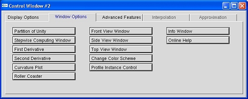
The Window Options tab provides all available windows.
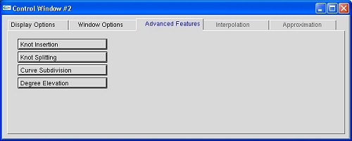
The Advanced Features tab shows the advanced features that are current available in version 2.
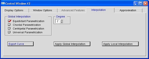
The Interpolation tab is available only if a user clicks on the The Start Interpolation button of the Control Window #1. It permits a user to select the way of computing parameters, a degree, and global or local interpolation.
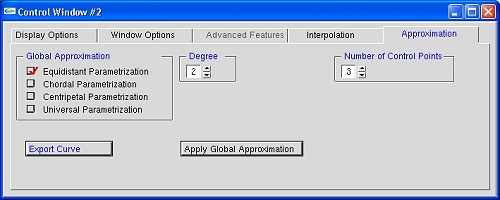
Similarly, the Approximation tab permits a user to select a way of computing parameters, a degree and the number of control points for the approximation B-spline curve.
Options and features in each of these five tabs will be added when they will become ready for testing.
This is essentially the version 1 surface system. Please note that the cross section design component is currently not very stable, and further development is needed. On the other hand, since we have found throughout the years that few people would use this component in classroom, we do not consider this problem significant.
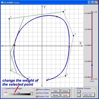
This small program is designed to help understand the concept of NURBS. Click here to learn the definition of NURBS and its geometric interpretation. A 3D NURBS curve can be obtained by projecting a 4D B-spline curve to 3D. Since it is difficult to show a 4D B-spline, this program shows the result of projecting a 3D B-spline to a plane to obtain a 2D NURBS curve.
This program has two windows: 2D NURBS Curve window and 3D-B-Spline-Projection window. A user can right-click the 2D NURBS Curve window to add control points, left-click to select a control point, and left-drag to move a control point. The created curve is a 2D B-spline curve (i.e., all weights being 1). Then, a user can select a control point and use the slide in the lower-left corner of the 2D NURBS Curve window to increase/decrease its weight. As the weight is being changed, the B-spline curve becomes a NURBS curve, and the 3D-B-Spline-Projection window shows the projection between a 3D-B-spline and its corresponding 2D NURBS curves.
|
|
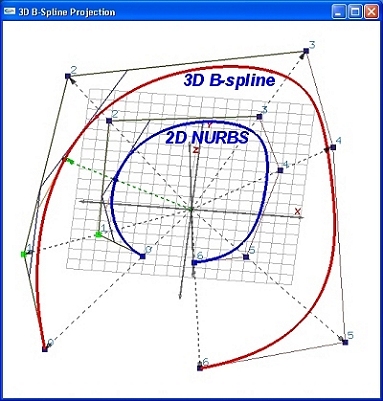
A user can use trackball technique to rotate the curves in the 3D B-Spline-Projection window. Moreover, a user may display de Boor net, which is shown in both windows. As a user traces the curve, the projection of the de Boor net of the 3D B-spline curve to the 2D NURBS can clearly be seen. The wight of a control point should not be negative because it will cause the strong convex hull property to fail.
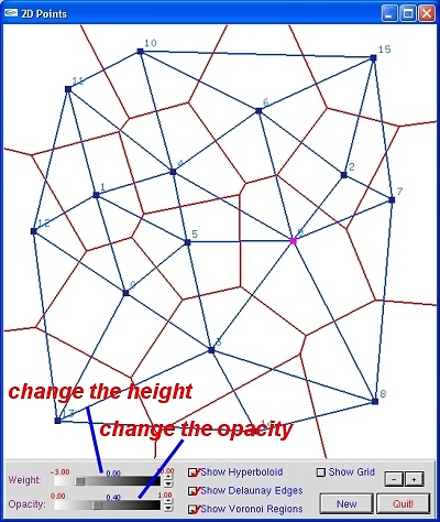
This program shows the relationship among 3D convex hull, 2D Voronoi region and 2D Delauney triangulation using two windows: 2D Points and 3D Projection. A user can right-click to add points to 2D Points window, left-click to select and left-drag to move a point. Each point (x,y) is mapped to the surface of a elliptic paraboloid z = (x2 + y2) + w, where w is a value that can be changed by the top slide in the lower left corner of the 2D Points window. Then, the 3D convex hull of these points is computed. The projection of the "lower" edges of this convex hull gives the Delauney triangulation. Connecting the two centers of circumcircle of the adjacent triangles yields the edges of the Voronoi region.
|
|
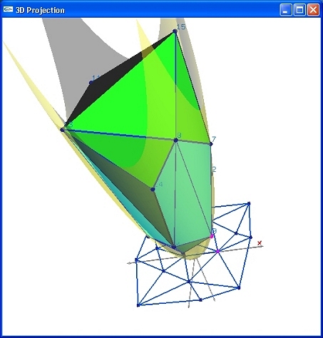
The 3D Projection shows the convex hull, Delauney triangulation and elliptic paraboloid. The whole configuration can be rotated with trackball technique. Moreover, a user can change the opacity of the paraboloid with the bottom slide in the lower-left corner of the 2D Points window.
If some items cannot be seen or a curve is not shown when the number of control points is larger than a small number (e.g., seven), please disable the hardware acceleration of your graphics card.
Please send your comments, suggestions, criticisms and bug-reports to shene@mtu.edu.