Short Tutorial on Using Spreadsheet to Obtain
Txy
Diagrams
(T.B.Co 10/29/2001)
Introduction
The calculations for bubble point temperature and dew point temperature
of an ideal binary mixture usually require numerical methods to aid in
determining the required values. In this tutorial, we show the use of the
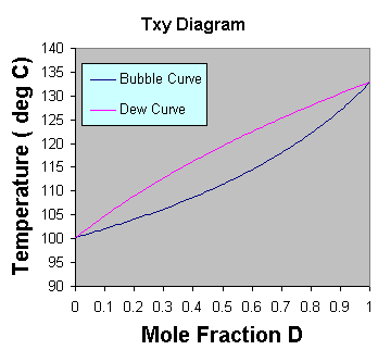
SOLVER utility of the Excel Spreadsheet program to obtain the curves for
a Txy diagram, i.e. the Bubble Point Curve and the Dew Point Curve. We
will also assume that Raoult's law applies and use the Antoine equation
to obtain the vapor pressures.
Procedure
(The example used in this tutorial will focus on a fictitious mixture
of compound D and compound E. The objective is to obtain the Txy diagram
for a fixed pressure of P=1 atm, with mole fraction D as the independent
variable. A zipped file of the example used below can be obtained
throught the link http://www.chem.mtu.edu/~tbco/cm2110/txy.zip.)
-
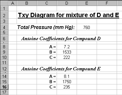
Setup the spreadsheet with the necessary parameters, e.g.
the pressure, the Antoine coefficients, etc.

-
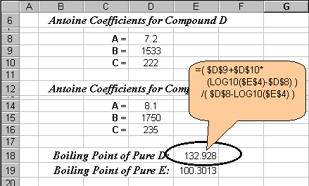
Solve for the boiling points of pure compounds. ( These will
be used to generate initial guesses later on ).
Based on Antoine equation, the boiling point for pure D is given
by

where AD, BD and CD are
the Antoine coefficients for compound D.

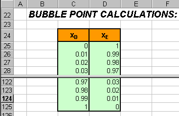
Bubble Point Calculations:
-
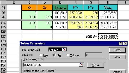
Setup the column for mole fraction D, mole fraction E.

-
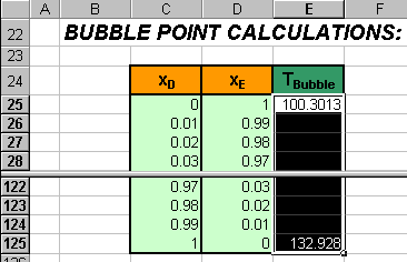
Create a column to contain the Bubble Point Temperatures.
First fill in the values for boiling points of pure B and pure E ( if using
COPY, be sure to use PASTE SPECIAL
and select VALUES option. )

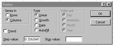
Next, mark the entries in the T-bubble column and then select from the
EDIT menu, the FILL then SERIES
item. A window should pop out. Choose
to fill the column using the linear type.

this should result in linearly interpolated data to be used as initial
guesses for bubble temperature.
-
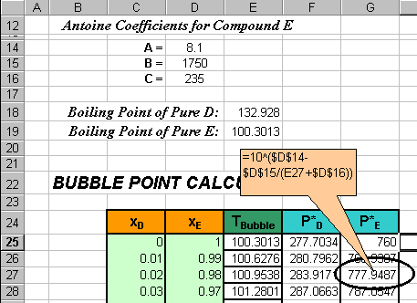
Calculate the corresponding vapor pressures of D and E using Antoine equation.

-
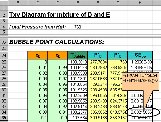
Generate a column that calculates the square of the error function for
the bubble temperature equation given by:

( Squaring the error means we deal with positive values. Thus the objective
will be to try and minimize these SE values.)

-
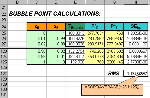
Calculate the RMS (root mean squared error). Create a cell
that calculate the square root of the average of all the squared errors.
This will monitor the accuracy of the bubble point curve using a single
average number. (The square root is simply to change the order of magnitude
back to the order of magnitudes of the errors prior to squaring them. )

-
Minimize the RMS value by changing Tbubble values.
Under the TOOLS menu, select the SOLVER item. A window should appear. Choose
to minimize the RMS (i.e. set the target cell address) by allowing the
SOLVER package to vary the cell value in the Tbubble
column (i.e. set cell addresses in the "By Changing Cells:" input). Then
click the SOLVE button.

-
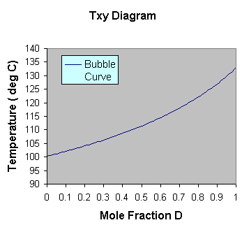
Plot the Tbubble curve.

Dew Point Calculations:
-
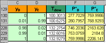
Set up the table. Follow steps similar to steps 3 to 5 with
the exception of using the labels yD, yE and Tdew
instead of xD, xE and Tbubble, respectively.

-
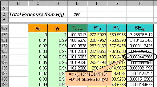
Generate a column that calculates the square of the error function for
the dew point temperature equation given by:


-
Create another RMS cell, this time for SEdp.
-
Minimize the RMS for SEdp using SOLVER.
-
Plot the resulting dew point curve along with bubble curve in the
previous graph.

This page is maintained by Tomas B. Co (tbco@mtu.edu).
Last revised 10/29/2001.
Tomas B. Co
Associate Professor
Department of Chemical Engineering
Michigan Technological University
1400 Townsend Avenue
Houghton, MI 49931-1295
Back to Homepage
