
To compute tangent and normal vectors at a point on a Bézier curve, we must compute the first and second derivatives at that point. Fortunately, computing the derivatives at a point on a Bézier curve is easy.
Recall that the Bézier curve defined by n + 1 control points P0, P1, ..., Pn has the following equation:
where Bn,i(u) is defined as follows:
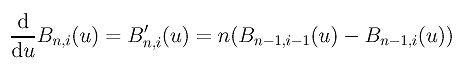
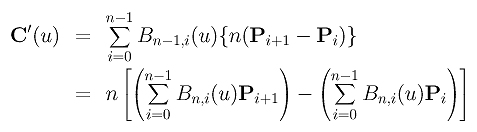
Since the control points are constants and independent of the variable u, computing the derivative curve C'(u) reduces to the computation of the derivatives of Bn,i(u)'s. With some simple algebraic manipulations, we have the following result for B'n,i(u):
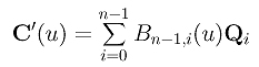
Then, computing the derivative of the curve C(u) yields:

Let Q0 = n(P1 - P0), Q1 = n(P2 - P1), Q2 = n(P3 - P2), ..., Qn-1 = n(Pn - Pn-1). The above equation reduces to the following:
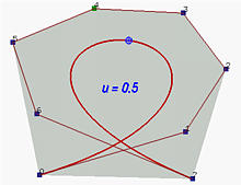
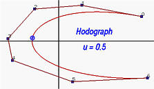
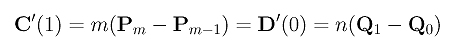
Therefore, the derivative of C(u) is a Bézier curve of degree n - 1 defined by n control points n(P1 - P0), n(P2 - P1), n(P3 - P2), ..., n(Pn - Pn-1). This derivative curve is usually referred to as the hodograph of the original Bézier curve. Note that Pi+1 - Pi is the direction vector from Pi to Pi+1 and n (Pi+1 - Pi) is n times longer than the direction vector. Once the control points are known, the control points of its derivative curve can be obtained immediately. The left figure below shows a Bézier curve of degree 7 and the right figure shows its derivative which is a degree 6 Bézier curve.

That a Bézier curve being tangent to its first and last legs provides us with a technique for joining two or more Bézier curves together for designing a desired shape. Let the first curve C(u) be defined by m + 1 control points P0, P1, P2, ..., Pm. Let the second curve D(u) be defined by n + 1 control points Q0, Q1, Q2, ..., Qn. If we want to join these two Bézier curves together, then Pm must be equal to Q0. This guarantees a C0 continuous join. Recall that the first curve is tangent to its last leg and the second curve is tangent to its first leg. Consequently, to achieve a smooth transition, Pm-1, Pm = Q0, and Q1 must be on the same line such that the directions from Pm-1 to Pm and the direction from Q0 to Q1 are the same. This is shown below.
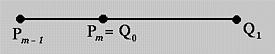
While joining two Bézier curves in this way looks smooth, it is still a C0 join and is not yet C1. However, it is G1, because they have the same tangent vector directions. To achieve C1 continuity, we have to make sure that the tangent vector at u = 1 of the first curve, C'(1), and the tangent vector at u = 0 of the second curve, D'(0), are identical. That is, the following must hold:
This relation states that to achieve C1 continuity at the joining point the ratio of the length of the last leg of the first curve (i.e., |pm - pm-1|) and the length of the first leg of the second curve (i.e., |q1 - q0|) must be n/m. Since the degrees m and n are fixed, we can adjust the positions of pm-1 or q1 on the same line so that the above relation is satisfied.
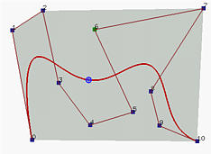
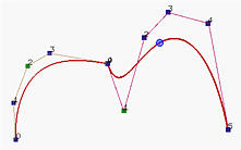
The left figure below has two Bézier curves. The light color polyline defines a Bézier curve of degree 4 while the dark color polyline defines a Bézier curve of degree 5. Since the last leg of the first curve and the first leg of the second are not on the same line, the two curves are not joint smoothly. The right figure shows two Bézier curves that are tangent to a line at the joining point. However, they are not C1 continuous. The left curve is of degree 4, while the right curve is of degree 7. But, the ratio of the last leg of the left curve and the first leg of the second curve seems near 1 rather than 7/4=1.75. To achieve C1 continuity, we should increase (resp., decrease) the length of the last (resp. first) leg of the left (resp., right). However, they are G1 continuous.

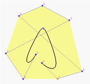
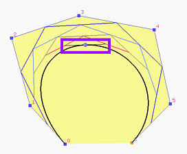
There is one more interesting application of this tangency property. If we let the first and last control points be identical (i.e., P0 = Pn) and P1, P0 and Pn-1 collinear, the generated Bézier curve will be a closed one and is G1 continuous at the joining point as shown below. To achieve C1 continuous at P0, we must have P1 - P0 = Pn - Pn-1 (i.e., the first and last legs have the same length and P1, P0 = Pn, Pn-1 are collinear)
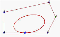
Note that although the above curve looks like an ellipse, it is not because this curve is of degree 6 and Bézier curves are polynomials which cannot represent circles and ellipses.
Thus, the derivative of a Bézier curve is the difference of two Bézier curves of degree n-1. For simplicity, let these two curves be C1(u) and C2(u):
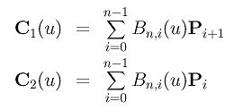
From these definitions, we know that the first curve C1(u) is defined by control points P1, P2, ..., Pn, that the second curve C2(u) is defined by control points P0, P1, ..., Pn-1, and that the derivative is:
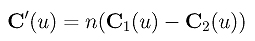
Therefore, theoretically, to compute the derivative of C(u) at a particular u, we can use de Casteljau's algorithm to compute C1(u) and C2(u). Then, computing their difference followed by multiplying by n yields C'(u). Therefore, the point on curve C(u) and its tangent vector C'(u) can be computed at the same time with de Casteljau's algorithm.
Now let us apply de Casteljau's algorithm to compute C1(u) and C2(u). See the figure below. The left-most column has all the given control points. The point n0 gives the point C(u) on the curve, and the segment joining (n-1)0 and (n-1)1 is the last control polyline of the de Casteljau net. In fact, n0 lies in the segment of (n-1)0 and (n-1)1 and divides it in a ratio of u:1-u.
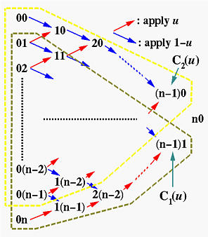
Since curve C1(u) is defined by control points 01, 02, ..., 0n, using the above diagram we know that (n-1)1 is the point on curve C1(u). Similarly, since C2(u) is defined by control points 00, 01, ..., 0(n-1), using the above diagram we know that (n-1)0 is the point on curve C2(u). Therefore, vector C1(u)-C2(u) is the vector from point (n-1)0 to point (n-1)1, and the derivative of C(u) is n times C1(u)-C2(u).
What does this mean? Since the line segment from (n-1)0 to (n-1)1 of the de Casteljau net has the same direction as the tangent vector at C(u), it is tangent to the curve at C(u)! In summary, we have
| The last polyline, actually a line segment, of a de Casteljau net is tangent to the Bézier curve at C(u). |
The following figure shows an example. The point shown corresponds to u = 0.5. It is clear that the last line segment of a de Casteljau net is tangent to C(0.5).
Applying the derivative formula to the above Bézier curve yields the following, which gives the second derivative of the original Bézier curve:
After obtaining C'(u) and C''(u), the moving triad and curvature at C(u) can be computed easily. Higher derivatives can be found by recursively applying the formula of derivative.
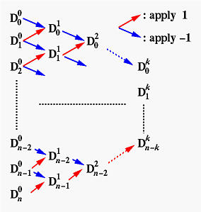
To express higher derivative concisely, we shall use finite difference. Let us define Di0 to be control point Pi for 0 <= i <= n. Then, we define the first level difference Di1 to be the difference of the previous level:
Note that the first level difference has only n points, one less than the number of given control points. More precisely, the first level of difference is the following:
The second level difference is defined to be the difference of the first level points:
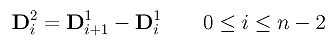
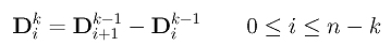
This second level difference has n-1 points. Repeating this procedure, we can define the k-th level difference as follows. The k-th level difference has n-k+1 point.
With these notation in hand, higher derivatives can be expressed concisely. First of all, let us rewrite C'(u) as follows, using the Di1's:
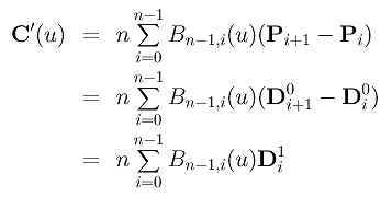
Applying the derivative to C'(u) to compute C''(u) gives us a formula of C''(u) in Di2's:
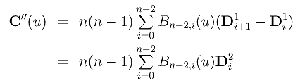
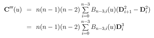
Do the same to C''(u) and we have a formula of C'''(u) in Di3's:
Continue this process and we can compute the k-th derivative C[k](u) in Dik's:

Therefore, to compute the k-th derivative of C(u) at a particular u, we first compute the Dik's and apply de Casteljau's algorithm to compute the point corresponding to u on the Bézier curve defined by Dik's. More precisely, we can arrange all Di0's on column 0, assign the south-east and north-east arrows -1 and 1, respectively, to compute column 1 of Di1's. Repeat this until we reach column k as shown below:
Finally, applying de Casteljau's algorithm to the points on column k with u and multiply the result by n(n-1)(n-2)...(n-k+1) gives us the vector of C[k](u)!