Item Response Theory
Fitting subject parameters in logistic regression
In a regression model, it is common to include participant as a predictor variable to account for overall individual variability, and this is essentially how mixed-effects models work when you give subject a random intercept. Suppose that you have a test with ten questions, and with individual variability across 50 individuals. Also, let’s suppose that each question has a different difficulty.
For participant j and question i, rather than a standard linear regression, logistic regression might be better, which models linear effects of the log-odds of a response being correct. We can think about the log-odds of successfully answering a question as being related to both the difficulty of the question and the ability of the person. The simplest version of this would be to take a factor \(\theta_j\) related to the ability of the person and add to it a value related to the easiness of each question. This is the same as subtracting \(b_i\)–something related to the difficulty of a question. So, a linear prediction in log-odds space would be (\(\theta_j -b_i\))
logodds <- function(p) {
    log(p/1 - p)
}  ##The probability of a 'yes' for a given set of predictor values.
logit <- function(lo) {
    1/(1 + exp(-lo))
}  ##This is the inverse of the logodds

set.seed(1009)
numsubs <- 50
numqs <- 20
skilllevel <- rnorm(numsubs)
questiondiff <- rnorm(numqs)
combined <- outer(skilllevel, questiondiff, function(x, y) {
    x - y
})
pcorrect <- logit(combined)
pcorrect.2 <- logit(combined + 2)  ## An easier test with the same subjects and problems.
Now, the matrix pcorrect indicates the probability of each person answering each question correctly. We can simulate a given experiment by comparing each probability value to a randomly chosen number uniformly between 0 and 1
Now, because this is all framed in terms of a log-odds an logistic transforms, we should be able to take the data in sim1 and estimate the parameters used to create them using logistic regression. To do so, we need to put the matrix in long format:
simdat <- data.frame(sub = factor(rep(1:numsubs, numqs)), question = factor(rep(1:numqs,
    each = numsubs)), corr = as.vector(sim1) + 0)

simdat.2 <- data.frame(sub = factor(rep(1:numsubs, numqs)), question = factor(rep(1:numqs,
    each = numsubs)), corr = as.vector(sim2) + 0)
Now, we just fit a logistic regression model. Because the baseline data had no intercept, we can re-estimate the parameters using a no-intercept model (specify +0 in the predictors)
Call:
glm(formula = corr ~ 0 + sub + question, family = binomial(),
    data = simdat)

Deviance Residuals:
    Min       1Q   Median       3Q      Max
-2.7131  -0.8781   0.2908   0.8382   2.3009

Coefficients:
           Estimate Std. Error z value Pr(>|z|)
sub1         3.5041     0.7518   4.661 3.14e-06 ***
sub2         1.1419     0.7397   1.544 0.122642
sub3         4.7411     0.9359   5.066 4.06e-07 ***
sub4         0.4008     0.8128   0.493 0.621959
sub5         4.7411     0.9359   5.066 4.06e-07 ***
sub6         5.5506     1.1788   4.709 2.49e-06 ***
sub7         4.2264     0.8377   5.045 4.53e-07 ***
sub8         3.8329     0.7844   4.886 1.03e-06 ***
sub9         2.2103     0.7030   3.144 0.001666 **
sub10        1.7097     0.7117   2.402 0.016290 *
sub11        3.2141     0.7306   4.399 1.09e-05 ***
sub12        4.2264     0.8377   5.045 4.53e-07 ***
sub13        2.4525     0.7039   3.484 0.000494 ***
sub14        3.2141     0.7306   4.399 1.09e-05 ***
sub15        3.2141     0.7306   4.399 1.09e-05 ***
 [ reached getOption("max.print") -- omitted 54 rows ]
---
Signif. codes:  0 '***' 0.001 '**' 0.01 '*' 0.05 '.' 0.1 ' ' 1

(Dispersion parameter for binomial family taken to be 1)

    Null deviance: 1386.3  on 1000  degrees of freedom
Residual deviance: 1009.8  on  931  degrees of freedom
AIC: 1147.8

Number of Fisher Scoring iterations: 16Analysis of Deviance Table
Model: binomial, link: logit
Response: corr
Terms added sequentially (first to last)
Df Deviance Resid. Df Resid. Dev Pr(>Chi)
NULL 1000 1386.3
sub 50 195.73 950 1190.6 < 2.2e-16 ***
question 19 180.72 931 1009.8 < 2.2e-16 ***
---
Signif. codes: 0 '***' 0.001 '**' 0.01 '*' 0.05 '.' 0.1 ' ' 1
Call:
glm(formula = corr ~ 0 + sub + question, family = binomial(),
    data = simdat.2)

Deviance Residuals:
     Min        1Q    Median        3Q       Max
-2.75946   0.00006   0.24361   0.49496   1.64680

Coefficients:
           Estimate Std. Error z value Pr(>|z|)
sub1          4.560      1.287   3.544 0.000394 ***
sub2          2.038      1.126   1.810 0.070318 .
sub3          5.346      1.468   3.641 0.000272 ***
sub4          4.059      1.220   3.327 0.000878 ***
sub5         21.895   2272.318   0.010 0.992312
sub6         21.895   2272.318   0.010 0.992312
sub7         21.895   2272.318   0.010 0.992312
sub8         21.895   2272.318   0.010 0.992312
sub9          5.346      1.468   3.641 0.000272 ***
sub10         2.788      1.141   2.442 0.014599 *
sub11         4.560      1.287   3.544 0.000394 ***
sub12         5.346      1.468   3.641 0.000272 ***
sub13         3.672      1.186   3.098 0.001951 **
sub14         4.059      1.220   3.327 0.000878 ***
sub15         4.560      1.287   3.544 0.000394 ***
 [ reached getOption("max.print") -- omitted 54 rows ]
---
Signif. codes:  0 '***' 0.001 '**' 0.01 '*' 0.05 '.' 0.1 ' ' 1

(Dispersion parameter for binomial family taken to be 1)

    Null deviance: 1386.29  on 1000  degrees of freedom
Residual deviance:  555.27  on  931  degrees of freedom
AIC: 693.27

Number of Fisher Scoring iterations: 18
We have a lack of identifiability here, because for any set of parameters, I can always add a constant to all subject parameters while subtracting it from all question parameters and obtain the same values. This can be seen in the model coefficients, which don’t have a question1. The performance on question1 is taken as a baseline, and all subject and question parameters are scaled to match it. We can use sum-to-zero contrasts and play with the intercept, and now our question coefficients will sum to 0, meaning the average difficulty of the questions has a log-odds of 0 (50% accuracy), easy questions have a positive coefficient, and difficult questions have a negative coefficient. Because we are fitting coefficients for each person, this does not mean the average accuracy of a question is 50%; for a relatively easy test, person-coefficients will be positive and for a hard test person-coefficients will be negative. Note that the subject coefficients have a similar interpretation: a person-coefficent of 0 means (when the item-coefficients sum to 0) means that that person is around 50% accurate overall, even though some items are harder and others are easier.
library(ggplot2)
library(tidyverse)
contrasts(simdat$question) <- contr.sum(levels(simdat$question))
contrasts(simdat.2$question) <- contr.sum(levels(simdat.2$question))

model <- glm(corr ~ 0 + sub + question, family = binomial(), data = simdat)
model2 <- glm(corr ~ 0 + sub + question, family = binomial(), data = simdat.2)


items <- data.frame(names = names(model$coefficients[51:69]), model1 = model$coefficients[51:69],
    model2 = model2$coefficients[51:69])


knitr::kable(items)| names | model1 | model2 | |
|---|---|---|---|
| question1 | question1 | 1.4387805 | 1.2641483 |
| question2 | question2 | -1.2205912 | -1.7364275 |
| question3 | question3 | -0.7084914 | -1.5774645 |
| question4 | question4 | 16.7194570 | 16.7384285 |
| question5 | question5 | -0.8126159 | -1.5774645 |
| question6 | question6 | -1.2205912 | -1.8882096 |
| question7 | question7 | -0.8126159 | 0.0491793 |
| question8 | question8 | -1.5257122 | -0.2971166 |
| question9 | question9 | -0.0378902 | -0.2971166 |
| question10 | question10 | -1.5257122 | -1.5774645 |
| question11 | question11 | -1.1192838 | 0.0491793 |
| question12 | question12 | -0.1574964 | -0.5792980 |
| question13 | question13 | 0.3526097 | -0.8211821 |
| question14 | question14 | -0.7084914 | -1.2299573 |
| question15 | question15 | -3.0993342 | -2.5814248 |
| question16 | question16 | -1.2205912 | -1.2299573 |
| question17 | question17 | -1.3219110 | 0.0491793 |
| question18 | question18 | -1.2205912 | -1.2299573 |
| question19 | question19 | -1.5257122 | -1.2299573 |
items %>%
    ggplot(aes(x = model1, y = model2)) + geom_point() + geom_abline(intercept = 0,
    slope = 1) + theme_bw() + ggtitle("Item parameters")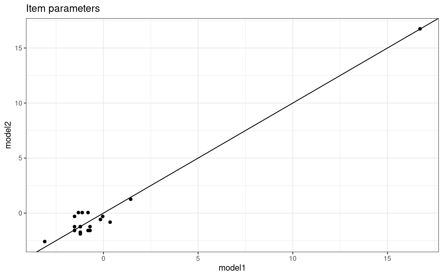
## Person coefficients

person <- data.frame(names = names(model$coefficients[1:50]), model1 = model$coefficients[1:50],
    model2 = model2$coefficients[1:50])


knitr::kable(person)| names | model1 | model2 | |
|---|---|---|---|
| sub1 | sub1 | 2.0653239 | 3.2956455 |
| sub2 | sub2 | -0.2968900 | 0.7736769 |
| sub3 | sub3 | 3.3023419 | 4.0819608 |
| sub4 | sub4 | -1.0379936 | 2.7946231 |
| sub5 | sub5 | 3.3023419 | 20.6306860 |
| sub6 | sub6 | 4.1118608 | 20.6306860 |
| sub7 | sub7 | 2.7876581 | 20.6306860 |
| sub8 | sub8 | 2.3940758 | 20.6306860 |
| sub9 | sub9 | 0.7715201 | 4.0819608 |
| sub10 | sub10 | 0.2709648 | 1.5234510 |
| sub11 | sub11 | 1.7752804 | 3.2956455 |
| sub12 | sub12 | 2.7876581 | 4.0819608 |
| sub13 | sub13 | 1.0136767 | 2.4081400 |
| sub14 | sub14 | 1.7752804 | 2.7946231 |
| sub15 | sub15 | 1.7752804 | 3.2956455 |
| sub16 | sub16 | 1.2576773 | 3.2956455 |
| sub17 | sub17 | 0.2709648 | 1.7917401 |
| sub18 | sub18 | -0.0001059 | 1.5234510 |
| sub19 | sub19 | 0.5258563 | 2.4081400 |
| sub20 | sub20 | 1.5092340 | 20.6306860 |
| sub21 | sub21 | 1.0136767 | 2.0820668 |
| sub22 | sub22 | 0.2709648 | 4.0819608 |
| sub23 | sub23 | 2.3940758 | 2.0820668 |
| sub24 | sub24 | -0.0001059 | 1.5234510 |
| sub25 | sub25 | -0.0001059 | 1.5234510 |
| sub26 | sub26 | 2.3940758 | 20.6306860 |
| sub27 | sub27 | 1.7752804 | 4.0819608 |
| sub28 | sub28 | 2.0653239 | 20.6306860 |
| sub29 | sub29 | -0.0001059 | 1.7917401 |
| sub30 | sub30 | 2.3940758 | 20.6306860 |
| sub31 | sub31 | 1.7752804 | 20.6306860 |
| sub32 | sub32 | 1.2576773 | 20.6306860 |
| sub33 | sub33 | 2.0653239 | 3.2956455 |
| sub34 | sub34 | 1.0136767 | 4.0819608 |
| sub35 | sub35 | 1.7752804 | 3.2956455 |
| sub36 | sub36 | 1.5092340 | 1.7917401 |
| sub37 | sub37 | -0.0001059 | 4.0819608 |
| sub38 | sub38 | 0.7715201 | 4.0819608 |
| sub39 | sub39 | 1.2576773 | 3.2956455 |
| sub40 | sub40 | 2.3940758 | 20.6306860 |
| sub41 | sub41 | 1.2576773 | 20.6306860 |
| sub42 | sub42 | 1.0136767 | 4.0819608 |
| sub43 | sub43 | 1.2576773 | 3.2956455 |
| sub44 | sub44 | 0.5258563 | 2.7946231 |
| sub45 | sub45 | -1.5647423 | 0.7736769 |
| sub46 | sub46 | 1.5092340 | 4.0819608 |
| sub47 | sub47 | -0.2968900 | 1.7917401 |
| sub48 | sub48 | -0.2968900 | 2.4081400 |
| sub49 | sub49 | 0.5258563 | 2.7946231 |
| sub50 | sub50 | 0.7715201 | 2.7946231 |
person %>%
ggplot(aes(x = model1, y = model2)) + geom_point() + geom_abline(intercept = 0,
slope = 1) + theme_bw() + ggtitle("Person parameters")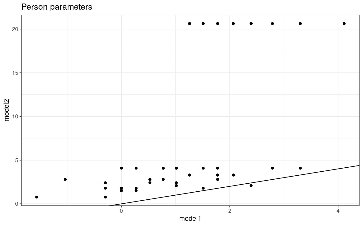 Notice that when framed this way, the item parameters estimate values
about the same, but the person parameters are different for the two
tests. The two regressions do not know about one another, so there is no
reason they should try to constrain the ability to be the same for each
person across the two tests, but this does raise the question of how
this should be done ideally, and how we should interpret these
paramaters in the wild. We might try to force the person parameters to
have an average of 0 and the items parameters to scale to fit the
difficulty of the test, which could make more sense.
Notice that when framed this way, the item parameters estimate values
about the same, but the person parameters are different for the two
tests. The two regressions do not know about one another, so there is no
reason they should try to constrain the ability to be the same for each
person across the two tests, but this does raise the question of how
this should be done ideally, and how we should interpret these
paramaters in the wild. We might try to force the person parameters to
have an average of 0 and the items parameters to scale to fit the
difficulty of the test, which could make more sense.
So, how good is it at recovering the parameters from which we created the data? Let’s compare our estimated parameters to our actual parameters:
library(ggplot2)
quickplot(x = model$coef[1:numsubs], y = skilllevel) + geom_point(size = 4) + xlab("Estimated Model coefficient") +
    ylab("Person Ability") + geom_label(label = 1:numsubs) + theme_bw()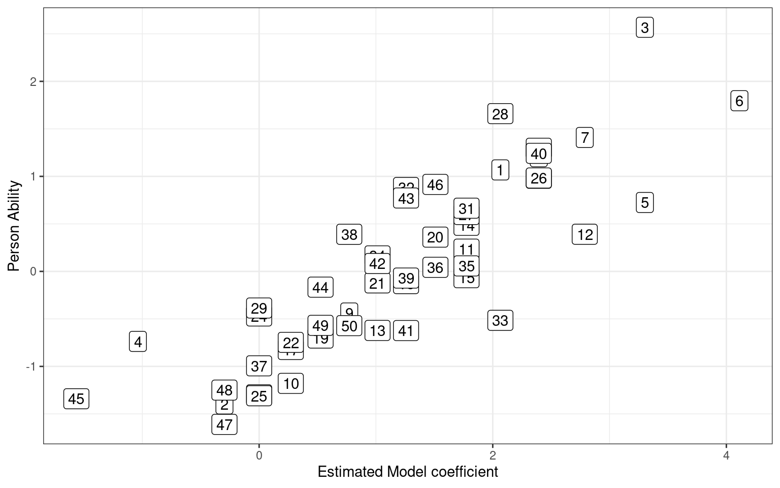
[1] 0.8558655This is not bad–we predict fairly well the skill level of each person based on 10 yes/no answers. How about assessing the question difficulty. In our sum-to-zero coding, question 20 is the negative average of the other items.
itempars <- c((model$coef[-(1:numsubs)]), -mean(model$coef[-(1:numsubs)]))
itempars2 <- c((model2$coef[-(1:numsubs)]), -mean(model2$coef[-(1:numsubs)]))

qplot(x = itempars, y = questiondiff) + geom_label(label = 1:length(questiondiff)) +
    xlab("Estimated Model coefficient") + ylab("Question difficulty") + theme_bw()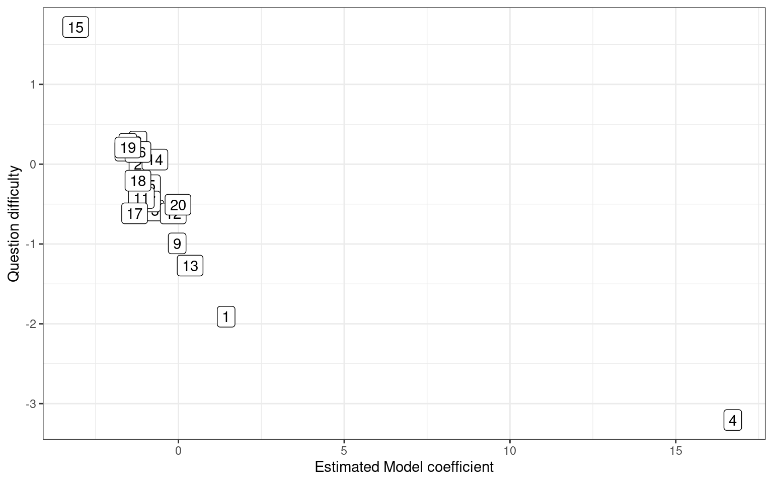
[1] -0.8104594We could have scored each person and each question according to accuracy:
 [1] 0.75 0.30 0.90 0.20 0.90 0.95 0.85 0.80 0.50 0.40 0.70 0.85 0.55 0.70 0.70
[16] 0.60 0.40 0.35 0.45 0.65 0.55 0.40 0.80 0.35 0.35 0.80 0.70 0.75 0.35 0.80
[31] 0.70 0.60 0.75 0.55 0.70 0.65 0.35 0.50 0.60 0.80 0.60 0.55 0.60 0.45 0.15
[46] 0.65 0.30 0.30 0.45 0.50 [1] 0.90 0.50 0.60 1.00 0.58 0.50 0.58 0.44 0.72 0.44 0.52 0.70 0.78 0.60 0.18
[16] 0.50 0.48 0.50 0.44 0.68grid.arrange(qplot(rowMeans(sim1), model$coef[1:numsubs], xlab = "Person accuracy",
ylab = "Person ability parameter") + theme_bw(), qplot(colMeans(sim1), itempars,
xlab = "Question accuracy", ylab = "Item difficulty parameter") + theme_bw(),
ncol = 2)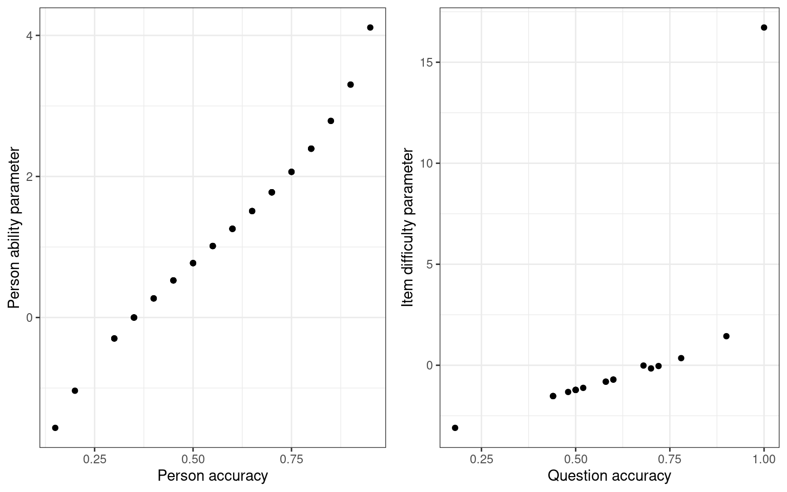
grid.arrange(qplot(rowMeans(sim2), model2$coef[1:numsubs], xlab = "Person accuracy",
    ylab = "Person ability parameter") + theme_bw(), qplot(colMeans(sim2), itempars2,
    xlab = "Question accuracy", ylab = "Item difficulty parameter") + theme_bw(),
    ncol = 2)
Notice that there is a fairly close mapping between the question
accuracy and the difficulty. What if we look at the two different tests
and compare parameter estimates:
Notice that there is a fairly close mapping between the question
accuracy and the difficulty. What if we look at the two different tests
and compare parameter estimates:
          set1      set2
set1 1.0000000 0.5772977
set2 0.5772977 1.0000000ggplot(abilities, aes(x = set1, y = set2)) + geom_point() + ggtitle("Person abilities") +
theme_bw()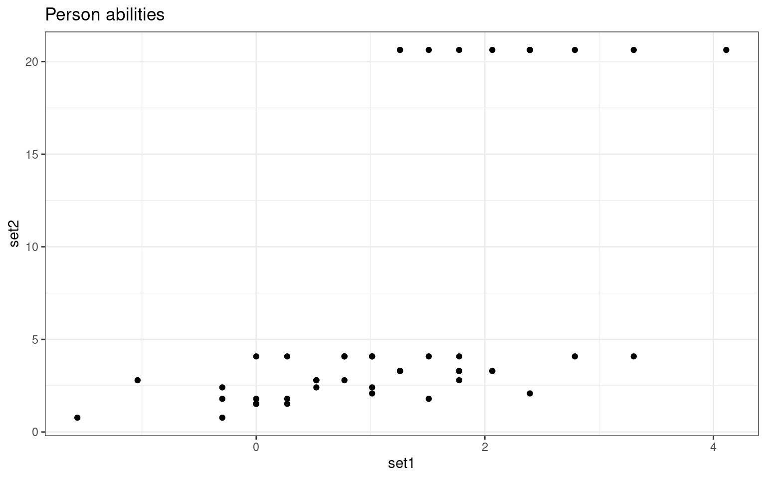
          set1      set2
set1 1.0000000 0.9841231
set2 0.9841231 1.0000000ggplot(probdifficulty, aes(x = set1, y = set2)) + geom_point() + ggtitle("Question difficulty") +
theme_bw()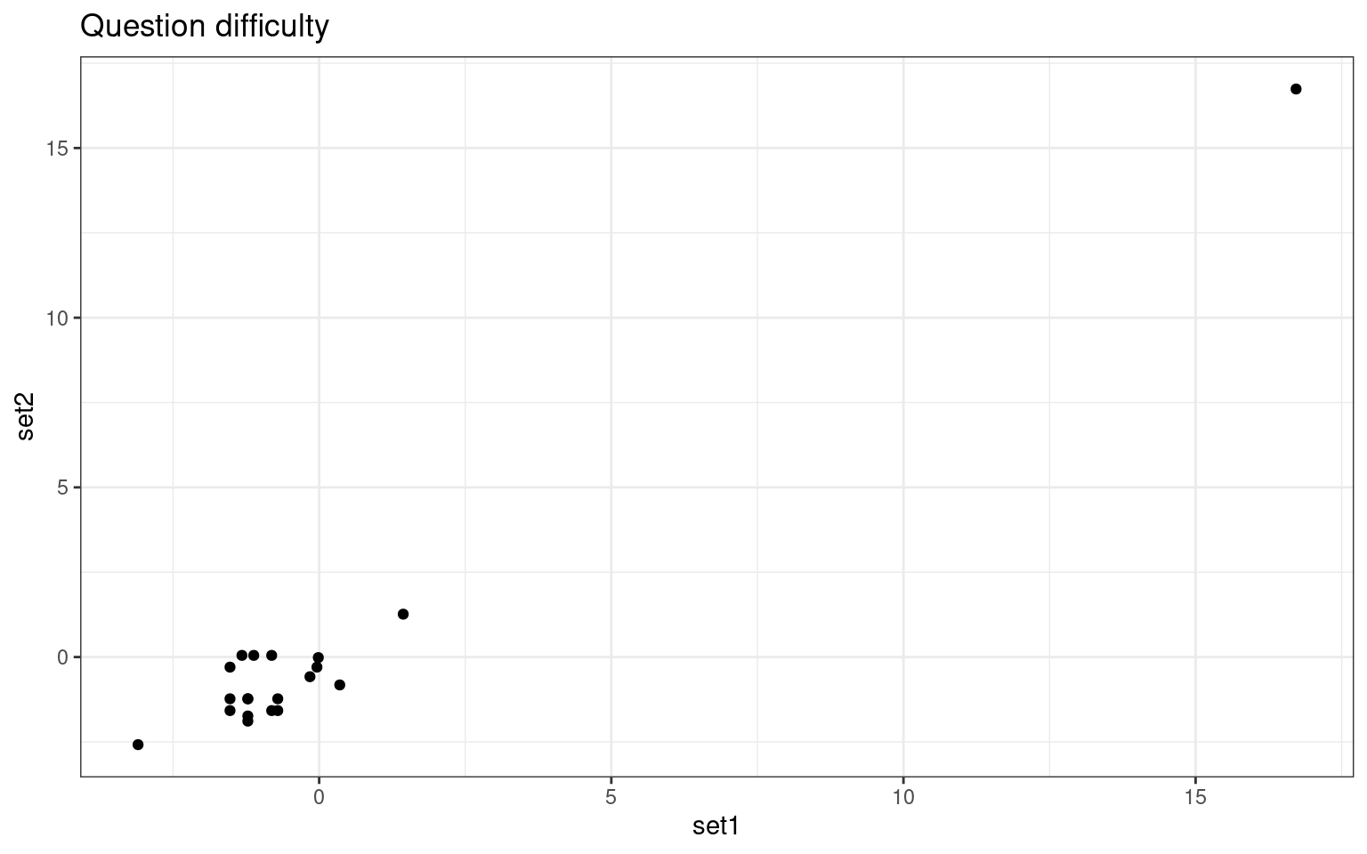 We are able to extract ‘person’ related coefficients across the two
tests that are reasonably well related. Furthermore, we get high
correlations for the test parameters
We are able to extract ‘person’ related coefficients across the two
tests that are reasonably well related. Furthermore, we get high
correlations for the test parameters
This analysis is essentially equivalent to what is known as the
Rasch model of Item Response Theory (IRT). The ltm
package estimates these directly from a wide data format. We might look
especially at how the Rasch model chooses to anchor difficulty
parameters.
library(ltm)

p1 <- sim1 + 0  #recode TF and 1/0
p2 <- sim2 + 0
irt1 <- rasch(p1)
irt2 <- rasch(p2)
summary(irt1)
Call:
rasch(data = p1)

Model Summary:
  log.Lik      AIC      BIC
 -565.682 1173.364 1213.517

Coefficients:
                  value    std.err  z.vals
Dffclt.Item 1   -2.6972     0.6433 -4.1927
Dffclt.Item 2    0.0009     0.3591  0.0026
Dffclt.Item 3   -0.5142     0.3703 -1.3888
Dffclt.Item 4  -28.3941 71439.4339 -0.0004
Dffclt.Item 5   -0.4094     0.3662 -1.1180
Dffclt.Item 6    0.0008     0.3591  0.0024
Dffclt.Item 7   -0.4095     0.3662 -1.1181
Dffclt.Item 8    0.3074     0.3630  0.8467
Dffclt.Item 9   -1.1912     0.4173 -2.8544
Dffclt.Item 10   0.3074     0.3630  0.8469
Dffclt.Item 11  -0.1009     0.3595 -0.2806
Dffclt.Item 12  -1.0699     0.4063 -2.6331
Dffclt.Item 13  -1.5870     0.4606 -3.4453
Dffclt.Item 14  -0.5143     0.3703 -1.3890
Dffclt.Item 15   1.8911     0.5009  3.7752
Dffclt.Item 16   0.0010     0.3591  0.0027
Dffclt.Item 17   0.1027     0.3595  0.2857
Dffclt.Item 18   0.0009     0.3591  0.0026
Dffclt.Item 19   0.3074     0.3630  0.8469
Dffclt.Item 20  -0.9533     0.3968 -2.4027
Dscrmn           0.9356     0.1343  6.9684

Integration:
method: Gauss-Hermite
quadrature points: 21

Optimization:
Convergence: 0
max(|grad|): 0.0019
quasi-Newton: BFGS
Call:
rasch(data = p2)

Model Summary:
   log.Lik      AIC      BIC
 -335.3924 712.7847 752.9372

Coefficients:
                  value    std.err  z.vals
Dffclt.Item 1   -3.7372     1.0006 -3.7349
Dffclt.Item 2   -1.3398     0.3768 -3.5559
Dffclt.Item 3   -1.4609     0.3917 -3.7292
Dffclt.Item 4  -21.8561 48471.2855 -0.0005
Dffclt.Item 5   -1.4608     0.3917 -3.7291
Dffclt.Item 6   -1.2254     0.3639 -3.3676
Dffclt.Item 7   -2.7467     0.6423 -4.2763
Dffclt.Item 8   -2.4679     0.5719 -4.3151
Dffclt.Item 9   -2.4674     0.5718 -4.3151
Dffclt.Item 10  -1.4609     0.3917 -3.7291
Dffclt.Item 11  -2.7455     0.6420 -4.2766
Dffclt.Item 12  -2.2411     0.5219 -4.2938
Dffclt.Item 13  -2.0490     0.4842 -4.2320
Dffclt.Item 14  -1.7281     0.4296 -4.0226
Dffclt.Item 15  -0.7187     0.3212 -2.2373
Dffclt.Item 16  -1.7277     0.4295 -4.0222
Dffclt.Item 17  -2.7448     0.6418 -4.2767
Dffclt.Item 18  -1.7277     0.4295 -4.0223
Dffclt.Item 19  -1.7277     0.4295 -4.0223
Dffclt.Item 20  -2.4680     0.5720 -4.3151
Dscrmn           1.2155     0.2000  6.0774

Integration:
method: Gauss-Hermite
quadrature points: 21

Optimization:
Convergence: 0
max(|grad|): 0.0053
quasi-Newton: BFGS
Descriptive statistics for the 'p1' data-set

Sample:
 20 items and 50 sample units; 0 missing values

Proportions for each level of response:
[[1]]
[1] 0.1 0.9

[[2]]
[1] 0.5 0.5

[[3]]
[1] 0.4 0.6

[[4]]
[1] 1

[[5]]
[1] 0.42 0.58

[[6]]
[1] 0.5 0.5

[[7]]
[1] 0.42 0.58

[[8]]
[1] 0.56 0.44

[[9]]
[1] 0.28 0.72

[[10]]
[1] 0.56 0.44

[[11]]
[1] 0.48 0.52

[[12]]
[1] 0.3 0.7

[[13]]
[1] 0.22 0.78

[[14]]
[1] 0.4 0.6

[[15]]
[1] 0.82 0.18

[[16]]
[1] 0.5 0.5

[[17]]
[1] 0.52 0.48

[[18]]
[1] 0.5 0.5

[[19]]
[1] 0.56 0.44

[[20]]
[1] 0.32 0.68


Frequencies of total scores:
     0 1 2 3 4 5 6 7 8 9 10 11 12 13 14 15 16 17 18 19 20
Freq 0 0 0 1 1 0 3 5 3 3  3  4  5  3  6  3  5  2  2  1  0


Cronbach's alpha:
                   value
All Items         0.7616
Excluding Item 1  0.7542
Excluding Item 2  0.7527
Excluding Item 3  0.7553
Excluding Item 4  0.7637
Excluding Item 5  0.7543
Excluding Item 6  0.7371
Excluding Item 7  0.7618
Excluding Item 8  0.7559
Excluding Item 9  0.7351
Excluding Item 10 0.7507
Excluding Item 11 0.7338
Excluding Item 12 0.7602
Excluding Item 13 0.7735
Excluding Item 14 0.7457
Excluding Item 15 0.7504
Excluding Item 16 0.7561
Excluding Item 17 0.7468
Excluding Item 18 0.7509
Excluding Item 19 0.7498
Excluding Item 20 0.7484


Pairwise Associations:
   Item i Item j p.value
1       1      8   1.000
2       1     12   1.000
3       1     13   1.000
4       1     15   1.000
5       1     18   1.000
6       1     19   1.000
7       2      4   1.000
8       2      7   1.000
9       2     13   1.000
10      2     18   1.000
Compare to our logistic regression:
plot(itempars, irt1$coef[, 1], main = "Comparison of model Item coefficients", xlab = "Logistic coefficients",
    ylab = "IRT coefficients")
abline(0, 1)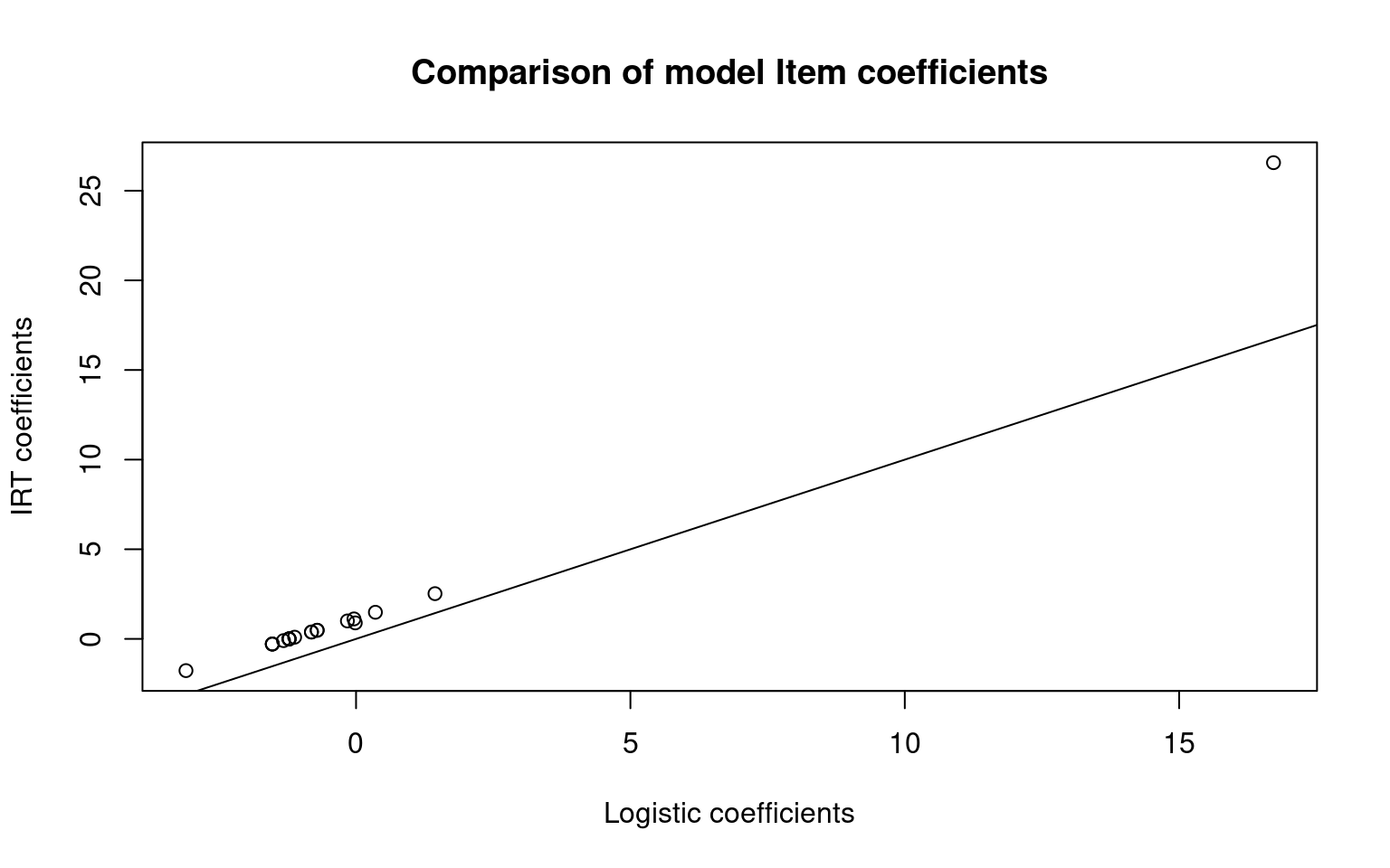
plot(itempars2, irt2$coef[, 1], main = "Comparison of model Item coefficients", xlab = "Logistic coefficients",
ylab = "IRT coefficients")
abline(0, 1)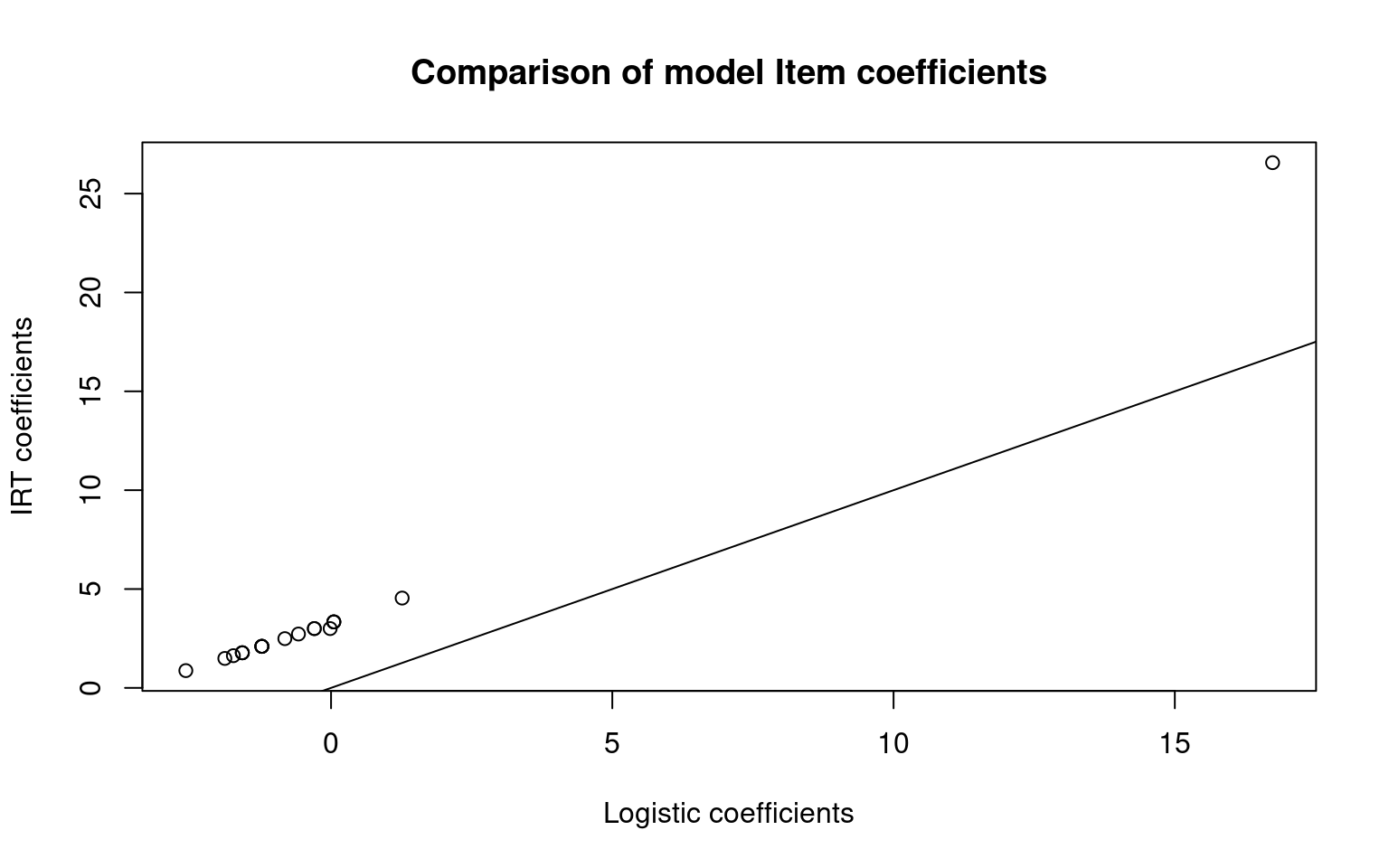 The item coefficients are not centered the same so their absolute values
are different. These models use person ability parameters, but do not
return those coefficients so it is not easy to make a direct comparison
to the logistic, or do a person-type analysis. Instead, the focus of IRT
is on the items or questions, which is usually what you care about; you
are often looking for a subset of items on a test that are especially
good, or to evaluate and remove bad items on a test.
The item coefficients are not centered the same so their absolute values
are different. These models use person ability parameters, but do not
return those coefficients so it is not easy to make a direct comparison
to the logistic, or do a person-type analysis. Instead, the focus of IRT
is on the items or questions, which is usually what you care about; you
are often looking for a subset of items on a test that are especially
good, or to evaluate and remove bad items on a test.
Visualizing the Rasch Model
If you plot() the model, it will display the inferred logistic curves for all the questions
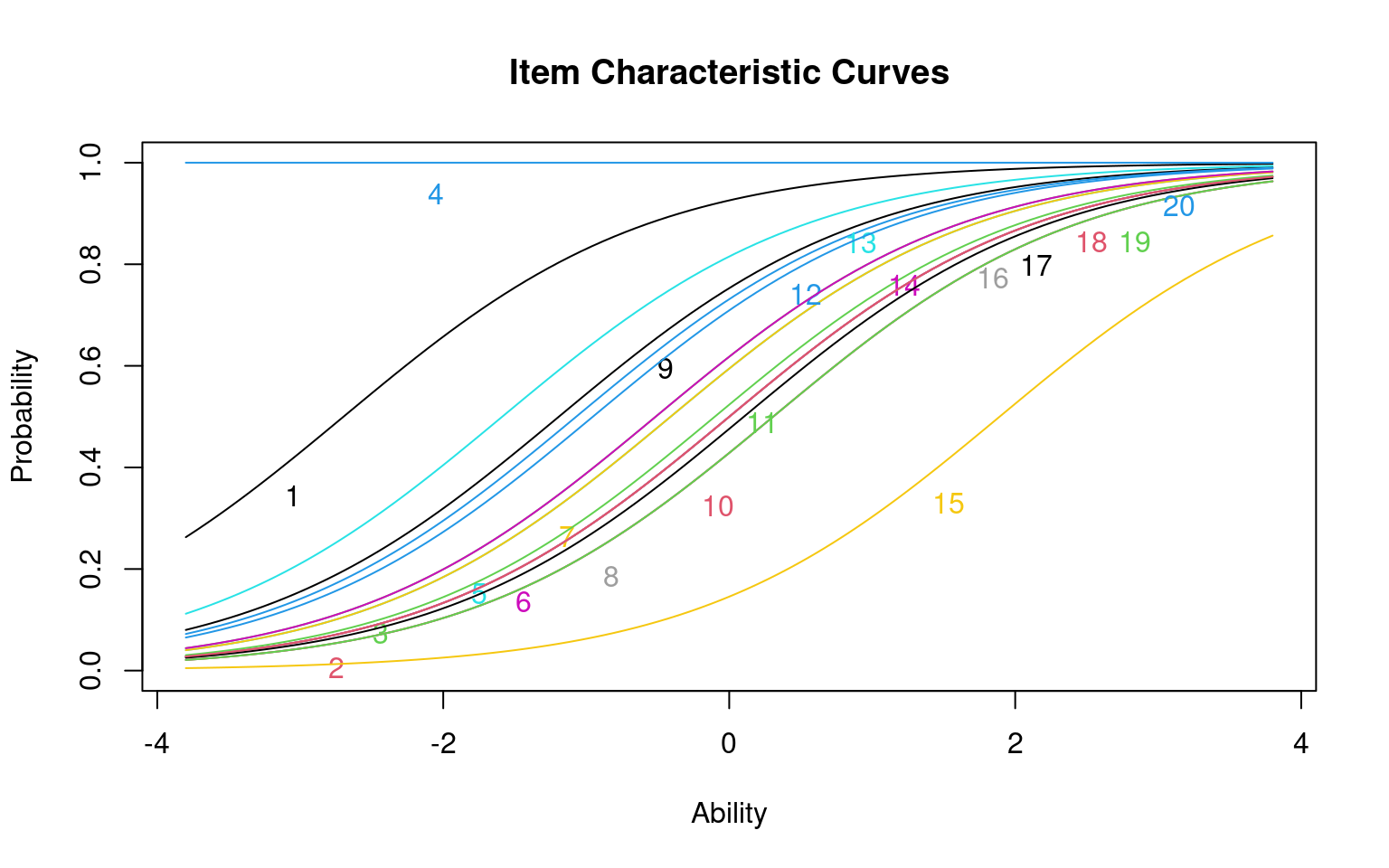
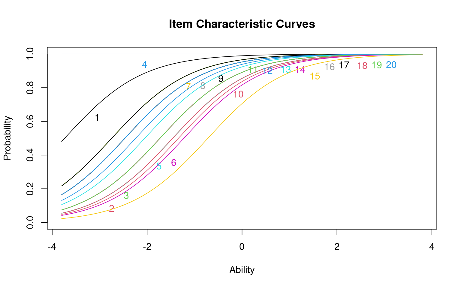
Notice that each curve is identical but shifted. The slope of the model is fit as a common value for all items, with different constant offsets (i.e., intercepts) for each question.
Boundary conditions of the Rasch Model
The data/questions in this example were all created as if they obeyed IRT. Thus, the model worked fairly well. If we have any violations of the model, the estimates can get less precise, and the small number of respondents (50) for the questions we chose (20) would not be enough. Typically you would want more, and the more complicated the model, the more participants.
What happens if they don’t–if we have ‘bad’ questions. One way to do this is to recode a few questions in the opposite direction, so that the people with high ability are more likely to get it wrong
set.seed(10010)
irt2 <- rasch(sim2 + 0)
sim3 <- sim2
sim3[, 1:5] <- (runif(5 * numsubs) < 0.5) + 0
irt3 <- rasch(sim3)
summary(irt2)
Call:
rasch(data = sim2 + 0)

Model Summary:
   log.Lik      AIC      BIC
 -335.3924 712.7847 752.9372

Coefficients:
                  value    std.err  z.vals
Dffclt.Item 1   -3.7372     1.0006 -3.7349
Dffclt.Item 2   -1.3398     0.3768 -3.5559
Dffclt.Item 3   -1.4609     0.3917 -3.7292
Dffclt.Item 4  -21.8561 48471.2855 -0.0005
Dffclt.Item 5   -1.4608     0.3917 -3.7291
Dffclt.Item 6   -1.2254     0.3639 -3.3676
Dffclt.Item 7   -2.7467     0.6423 -4.2763
Dffclt.Item 8   -2.4679     0.5719 -4.3151
Dffclt.Item 9   -2.4674     0.5718 -4.3151
Dffclt.Item 10  -1.4609     0.3917 -3.7291
Dffclt.Item 11  -2.7455     0.6420 -4.2766
Dffclt.Item 12  -2.2411     0.5219 -4.2938
Dffclt.Item 13  -2.0490     0.4842 -4.2320
Dffclt.Item 14  -1.7281     0.4296 -4.0226
Dffclt.Item 15  -0.7187     0.3212 -2.2373
Dffclt.Item 16  -1.7277     0.4295 -4.0222
Dffclt.Item 17  -2.7448     0.6418 -4.2767
Dffclt.Item 18  -1.7277     0.4295 -4.0223
Dffclt.Item 19  -1.7277     0.4295 -4.0223
Dffclt.Item 20  -2.4680     0.5720 -4.3151
Dscrmn           1.2155     0.2000  6.0774

Integration:
method: Gauss-Hermite
quadrature points: 21

Optimization:
Convergence: 0
max(|grad|): 0.0053
quasi-Newton: BFGS
Call:
rasch(data = sim3)

Model Summary:
   log.Lik      AIC      BIC
 -444.2396 930.4791 970.6316

Coefficients:
                 value std.err  z.vals
Dffclt.Item 1  -0.2581  0.4654 -0.5546
Dffclt.Item 2   0.3966  0.4693  0.8451
Dffclt.Item 3  -0.5225  0.4755 -1.0989
Dffclt.Item 4   0.2659  0.4652  0.5716
Dffclt.Item 5   0.3968  0.4693  0.8455
Dffclt.Item 6  -1.8679  0.6167 -3.0287
Dffclt.Item 7  -4.3637  1.1820 -3.6919
Dffclt.Item 8  -3.8917  1.0450 -3.7240
Dffclt.Item 9  -3.8921  1.0451 -3.7240
Dffclt.Item 10 -2.2409  0.6778 -3.3061
Dffclt.Item 11 -4.3638  1.1820 -3.6919
Dffclt.Item 12 -3.5111  0.9459 -3.7121
Dffclt.Item 13 -3.1954  0.8705 -3.6707
Dffclt.Item 14 -2.6720  0.7584 -3.5231
Dffclt.Item 15 -1.0778  0.5170 -2.0847
Dffclt.Item 16 -2.6712  0.7583 -3.5228
Dffclt.Item 17 -4.3641  1.1821 -3.6918
Dffclt.Item 18 -2.6713  0.7583 -3.5228
Dffclt.Item 19 -2.6720  0.7584 -3.5231
Dffclt.Item 20 -3.8914  1.0450 -3.7240
Dscrmn          0.6761  0.1298  5.2080

Integration:
method: Gauss-Hermite
quadrature points: 21

Optimization:
Convergence: 0
max(|grad|): 0.0072
quasi-Newton: BFGS plot((cbind(irt1$coef[, 1], irt3$coef[, 1])), main = "Item coefficients with bad questions",
xlab = "test 2", ylab = "test 3")
plot((cbind(irt1$coef[, 1], irt3$coef[, 1])), main = "Item coefficients with bad questions (zoomed)",
xlab = "test 2", ylab = "test 3", ylim = c(-5, 5))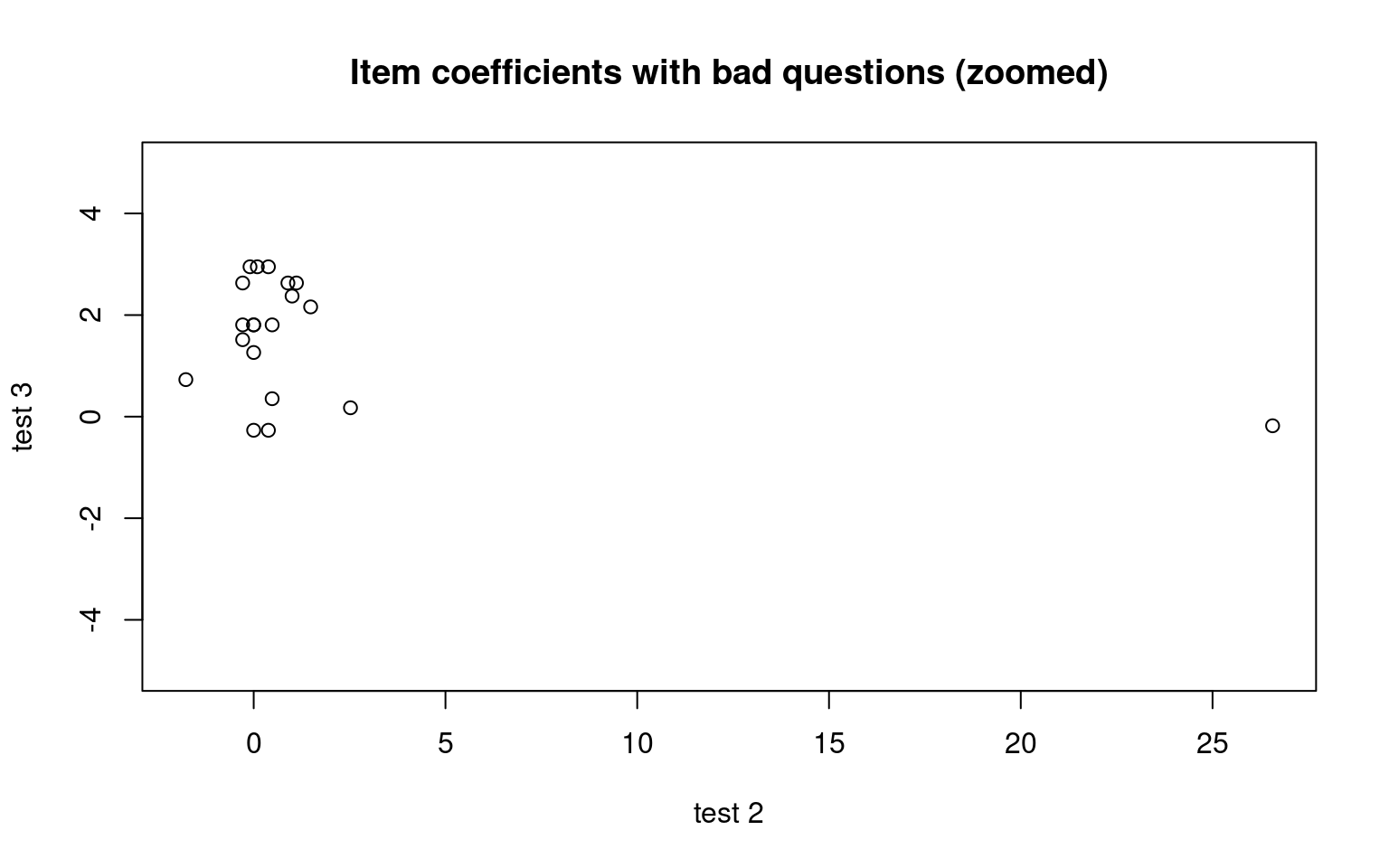 In this case, the ‘bad’ questions all ended up with negative difficulty
coefficients. If we examine the questions using item.fit, it will test
whether each question fits into the basic model. When everything was
from the model, none of the items were selected as bad. Once we made 5
items (25%) bad, in this case a bunch of items get flagged. This
includes all the items 1..5, but also 6, 7, and 9 and maybe 18.
Strangely, a few bad questions might make other questions look bad as
well.
In this case, the ‘bad’ questions all ended up with negative difficulty
coefficients. If we examine the questions using item.fit, it will test
whether each question fits into the basic model. When everything was
from the model, none of the items were selected as bad. Once we made 5
items (25%) bad, in this case a bunch of items get flagged. This
includes all the items 1..5, but also 6, 7, and 9 and maybe 18.
Strangely, a few bad questions might make other questions look bad as
well.
Item-Fit Statistics and P-values

Call:
rasch(data = sim2 + 0)

Alternative: Items do not fit the model
Ability Categories: 10

          X^2 Pr(>X^2)
It 1   2.4798   0.9286
It 2  13.5244   0.0603
It 3   5.2193   0.6332
It 4   0.0000        1
It 5  13.3812   0.0633
It 6   6.6327   0.4681
It 7   3.6856   0.8152
It 8   4.6883   0.6979
It 9  14.4979    0.043
It 10  8.9407   0.2569
It 11  6.8692   0.4426
It 12  5.4804   0.6016
It 13 10.4973   0.1621
It 14  4.3378   0.7401
It 15  5.0282   0.6565
It 16  8.0741   0.3261
It 17  7.3144   0.3969
It 18  7.9045   0.3411
It 19  9.9131   0.1936
It 20  4.0405   0.7751
Item-Fit Statistics and P-values

Call:
rasch(data = sim3)

Alternative: Items do not fit the model
Ability Categories: 10

          X^2 Pr(>X^2)
It 1   3.5064   0.7431
It 2   3.8323   0.6994
It 3   2.5409   0.8639
It 4   5.8604    0.439
It 5   8.6429   0.1947
It 6   3.9761   0.6799
It 7   4.3075   0.6351
It 8   7.5153   0.2758
It 9   3.8459   0.6975
It 10  5.2996    0.506
It 11  3.0357   0.8044
It 12  7.8566   0.2488
It 13  3.3830   0.7595
It 14  6.1092   0.4111
It 15 10.6329   0.1004
It 16  3.8659   0.6948
It 17 10.7470   0.0965
It 18  2.6317   0.8534
It 19  3.6177   0.7283
It 20  2.8663   0.8254
Some of the other things we can look at to examine the fit of the model:
Person-Fit Statistics and P-values

Call:
rasch(data = sim2 + 0)

Alternative: Inconsistent response pattern under the estimated model

  It 1 It 2 It 3 It 4 It 5 It 6 It 7 It 8 It 9 It 10 It 11 It 12 It 13 It 14
1    0    0    0    1    0    1    1    0    1     1     1     1     1     1
2    1    0    0    1    0    0    0    1    1     1     1     0     0     0
3    1    0    0    1    0    0    1    1    1     0     0     0     1     0
  It 15 It 16 It 17 It 18 It 19 It 20       L0      Lz Pr(<Lz)
1     0     1     1     0     1     1 -12.6539 -1.0533  0.1461
2     0     1     1     0     1     1 -10.8261  0.6039  0.7271
3     0     0     1     1     1     1 -10.1098  1.0793  0.8598
 [ reached 'max' / getOption("max.print") -- omitted 33 rows ]
Person-Fit Statistics and P-values

Call:
rasch(data = sim3)

Alternative: Inconsistent response pattern under the estimated model

  It 1 It 2 It 3 It 4 It 5 It 6 It 7 It 8 It 9 It 10 It 11 It 12 It 13 It 14
1    0    0    0    0    1    1    1    1    1     0     1     0     1     0
2    0    0    0    0    1    1    1    1    1     0     1     1     1     1
3    0    0    0    1    0    0    0    1    1     1     1     0     0     0
  It 15 It 16 It 17 It 18 It 19 It 20       L0      Lz Pr(<Lz)
1     1     0     1     1     0     1 -12.1349 -0.6812  0.2479
2     0     0     0     1     1     1 -10.9041 -0.2671  0.3947
3     0     1     1     0     1     1 -12.9750 -0.8758  0.1906
 [ reached 'max' / getOption("max.print") -- omitted 43 rows ]
Extending and Constraining IRT
Slope of the item characteristic function
In the Rasch model, all items are of the same family, and have the
same slope, or steepness. If this were a logistic regression, this would
be a coefficient on an item difficulty predictor—even though item
difficulty is itself a coefficient of the model. Or it is more like a
parameter on the binomial error distribution, and so maps onto the
quasi-binomial we used to estimate overdispersion. So this goes beyond
what we would easily be able to do in a simple logistic regression. For
the rasch model to do this, it uses the general-purpose
optim function, which has a number of optimization methods.
The ltm library uses Broyden-Fletcher-Goldfarb-Shanno (BFGS) method in
optim, and although others are available, rasch hard-codes
the method because BFGS works fairly well.
A very steep function means that there is a sharp cut-off between who can answer it correctly and who cannot. This is often called ‘discriminability’. A good test item typically has high discriminability, and a good test has a set of highly-discriminable items that have different difficulty. Typically, high discriminability will correspond to good part-whole item correlations. As a sort of ideal situation, the easiest item will be answered correctly by everyone but the lowest-ability person, the hardest item will only be answered correctly by the highest-ability person, and the person’s ability will directly control how many of the items they can answer. As a rule of thumb, higher discriminability values (greater than 1.0, or better yet greater than 2.0) are good. By default, the rasch model estimates a slope. However, the default logistic model will have a slope of 1.0, and so this is sometimes considered a simpler model. You might do this if you have limited data–maybe a test from a class with relatively few students, because it will hopefully make estimation more stable.
For example, The following is are the results of a psychology test:
dat <- read.csv("testscores.csv")

## descript(dat) ##doesn't work. Thus compute Cronbach's alpha on the data
descript(dat, chi.squared = F)
Descriptive statistics for the 'dat' data-set

Sample:
 47 items and 21 sample units; 0 missing values

Proportions for each level of response:
$q1
1
1

$q2
     0      1
0.3333 0.6667

$q3
1
1

$q4
     0      1
0.8095 0.1905

$q5
     0      1
0.1429 0.8571

$q6
     0      1
0.3333 0.6667

$q7
     0      1
0.2381 0.7619

$q8
     0      1
0.1429 0.8571

$q9
1
1

$q10
     0      1
0.0476 0.9524

$q11
    0     1
0.619 0.381

$q12
    0     1
0.381 0.619

$q13
     0      1
0.0476 0.9524

$q14
1
1

$q15
     0      1
0.7619 0.2381

$q16
     0      1
0.0476 0.9524

$q17
1
1

$q18
     0      1
0.0476 0.9524

$q19
     0      1
0.3333 0.6667

$q20
     0      1
0.2381 0.7619

$q21
1
1

$q22
     0      1
0.2857 0.7143

$q23
     0      1
0.2381 0.7619

$q24
1
1

$q25
     0      1
0.6667 0.3333

$q26
1
1

$q27
     0      1
0.7143 0.2857

$q28
    0     1
0.381 0.619

$q29
    0     1
0.381 0.619

$q31
     0      1
0.6667 0.3333

$q32
     0      1
0.6667 0.3333

$q33
     0      1
0.4762 0.5238

$q34
     0      1
0.0952 0.9048

$q35
     0      1
0.3333 0.6667

$q36
    0     1
0.619 0.381

$q37
     0      1
0.3333 0.6667

$q38
     0      1
0.1905 0.8095

$q39
     0      1
0.7619 0.2381

$q40
     0      1
0.4762 0.5238

$q41
     0      1
0.0476 0.9524

$q42
     0      1
0.1429 0.8571

$q43
     0      1
0.0952 0.9048

$q44
    0     1
0.381 0.619

$q45
    0     1
0.381 0.619

$q47
     0      1
0.2381 0.7619

$q48
    0     1
0.619 0.381

$q49
     0      1
0.7143 0.2857


Frequencies of total scores:
     0 1 2 3 4 5 6 7 8 9 10 11 12 13 14 15 16 17 18 19 20 21 22 23 24 25 26 27
Freq 0 0 0 0 0 0 0 0 0 0  0  0  0  0  0  0  0  0  0  0  0  0  0  0  0  0  0  3
     28 29 30 31 32 33 34 35 36 37 38 39 40 41 42 43 44 45 46 47
Freq  0  2  3  3  2  1  1  1  0  0  1  3  0  1  0  0  0  0  0  0


Cronbach's alpha:
               value
All Items     0.6291
Excluding q1  0.6294
Excluding q2  0.6504
Excluding q3  0.6294
Excluding q4  0.6317
Excluding q5  0.6138
Excluding q6  0.5851
Excluding q7  0.6021
Excluding q8  0.6313
Excluding q9  0.6294
Excluding q10 0.6211
Excluding q11 0.6217
Excluding q12 0.6122
Excluding q13 0.6297
Excluding q14 0.6294
Excluding q15 0.6309
Excluding q16 0.6254
Excluding q17 0.6294
Excluding q18 0.6297
Excluding q19 0.5979
Excluding q20 0.6139
Excluding q21 0.6294
Excluding q22 0.6342
Excluding q23 0.6251
Excluding q24 0.6294
Excluding q25 0.6426
Excluding q26 0.6294
Excluding q27 0.6118
Excluding q28 0.5952
Excluding q29 0.6168
Excluding q31 0.6124
Excluding q32 0.6147
Excluding q33 0.6177
Excluding q34 0.6232
Excluding q35 0.6302
Excluding q36 0.6526
Excluding q37 0.6406
Excluding q38 0.6174
Excluding q39 0.6200
Excluding q40 0.6107
Excluding q41 0.6317
Excluding q42 0.6334
Excluding q43 0.6337
Excluding q44 0.6075
Excluding q45 0.6425
Excluding q47 0.6116
Excluding q48 0.6428
Excluding q49 0.6047
# force the discrimination parameter to be 1
model1 <- rasch(dat, constraint = cbind(length(dat) + 1, 1))
model1
Call:
rasch(data = dat, constraint = cbind(length(dat) + 1, 1))

Coefficients:
 Dffclt.q1   Dffclt.q2   Dffclt.q3   Dffclt.q4   Dffclt.q5   Dffclt.q6
   -25.566      -0.773     -25.566       1.591      -1.947      -0.773
 Dffclt.q7   Dffclt.q8   Dffclt.q9  Dffclt.q10  Dffclt.q11  Dffclt.q12
    -1.281      -1.946     -25.566      -3.188       0.531      -0.546
Dffclt.q13  Dffclt.q14  Dffclt.q15  Dffclt.q16  Dffclt.q17  Dffclt.q18
    -3.188     -25.566       1.281      -3.188     -25.566      -3.188
Dffclt.q19  Dffclt.q20  Dffclt.q21  Dffclt.q22  Dffclt.q23  Dffclt.q24
    -0.773      -1.281     -25.566      -1.016      -1.281     -25.566
Dffclt.q25  Dffclt.q26  Dffclt.q27  Dffclt.q28  Dffclt.q29  Dffclt.q31
     0.762     -25.566       1.009      -0.545      -0.546       0.762
Dffclt.q32  Dffclt.q33  Dffclt.q34  Dffclt.q35  Dffclt.q36  Dffclt.q37
     0.762      -0.114      -2.425      -0.773       0.531      -0.773
Dffclt.q38  Dffclt.q39  Dffclt.q40  Dffclt.q41  Dffclt.q42  Dffclt.q43
    -1.583       1.281      -0.115      -3.188      -1.946      -2.424
Dffclt.q44  Dffclt.q45  Dffclt.q47  Dffclt.q48  Dffclt.q49      Dscrmn
    -0.546      -0.545      -1.281       0.531       1.009       1.000

Log.Lik: -430.349
Call:
rasch(data = dat)

Coefficients:
 Dffclt.q1   Dffclt.q2   Dffclt.q3   Dffclt.q4   Dffclt.q5   Dffclt.q6
   -49.028      -1.416     -49.028       2.930      -3.615      -1.418
 Dffclt.q7   Dffclt.q8   Dffclt.q9  Dffclt.q10  Dffclt.q11  Dffclt.q12
    -2.362      -3.612     -49.028      -5.965       0.984      -0.996
Dffclt.q13  Dffclt.q14  Dffclt.q15  Dffclt.q16  Dffclt.q17  Dffclt.q18
    -5.966     -49.028       2.361      -5.967     -49.028      -5.966
Dffclt.q19  Dffclt.q20  Dffclt.q21  Dffclt.q22  Dffclt.q23  Dffclt.q24
    -1.417      -2.364     -49.028      -1.869      -2.362     -49.028
Dffclt.q25  Dffclt.q26  Dffclt.q27  Dffclt.q28  Dffclt.q29  Dffclt.q31
     1.407     -49.028       1.862      -0.996      -0.996       1.408
Dffclt.q32  Dffclt.q33  Dffclt.q34  Dffclt.q35  Dffclt.q36  Dffclt.q37
     1.408      -0.206      -4.517      -1.416       0.984      -1.416
Dffclt.q38  Dffclt.q39  Dffclt.q40  Dffclt.q41  Dffclt.q42  Dffclt.q43
    -2.928       2.361      -0.201      -5.966      -3.612      -4.518
Dffclt.q44  Dffclt.q45  Dffclt.q47  Dffclt.q48  Dffclt.q49      Dscrmn
    -0.996      -0.996      -2.364       0.984       1.862       0.521

Log.Lik: -426.767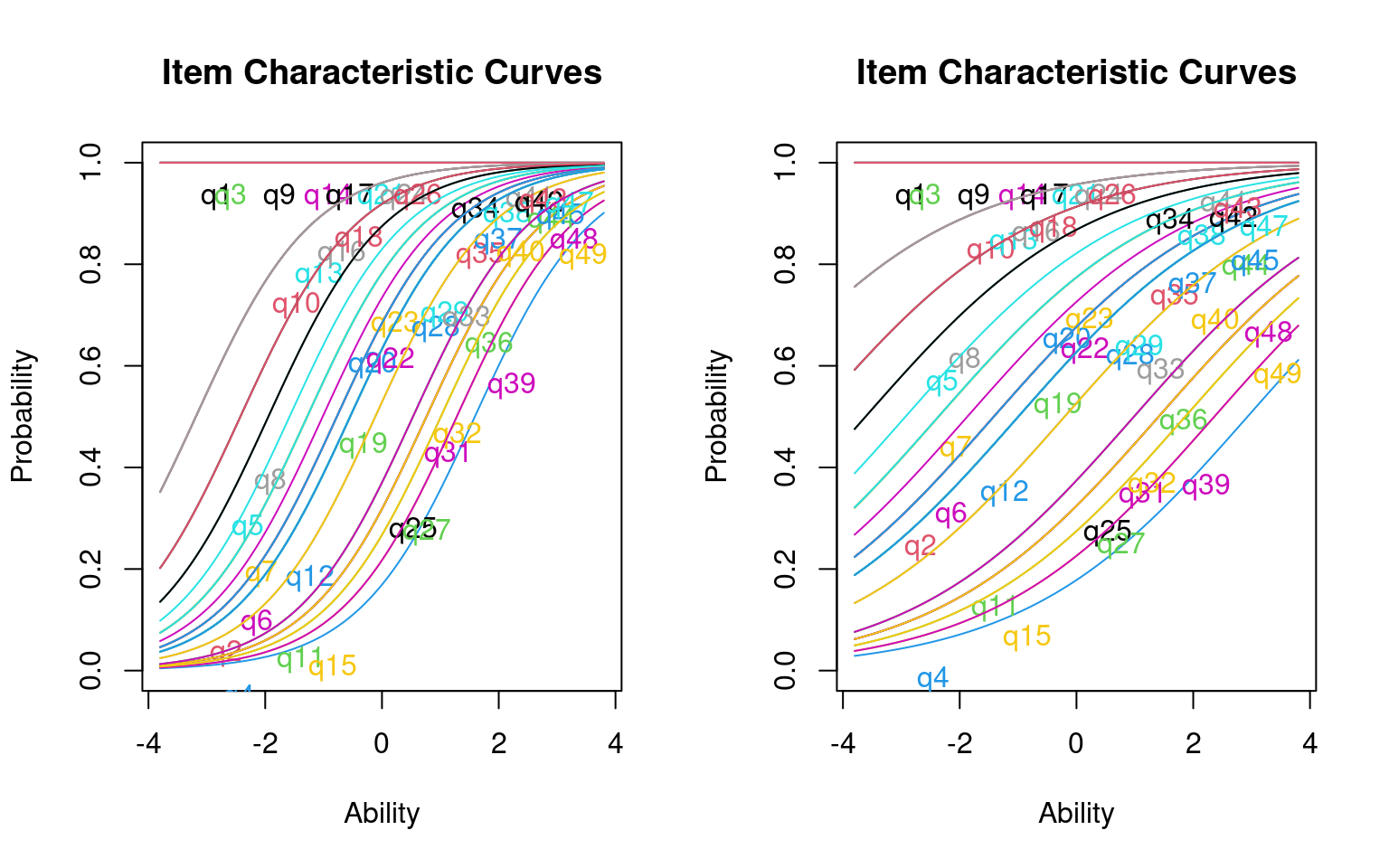
Notice that several of the questions have difficulty parameters of -49.02. These are the problems that everybody got correct. This also likely led to the error messages returned by the models. It is difficult to estimate the difficulty of such questions, because they must be really easy. We fit two different models; one in which has a discrimination parameter. Is it worthwhile using this extra parameter?
 Likelihood Ratio Table
          AIC     BIC log.Lik  LRT df p.value
model1 954.70 1003.79 -430.35
model2 949.53  999.67 -426.77 7.16  1   0.007
Results show that there is no difference between the two, despite the fact that the mean discriminability when estimated was .5 instead of 1; however model1 had lower AIC and BIC scores resulting from a higher (less negative) log-likelihood.
Fitting individual difficulty parameters
In other cases, it is likely that different items have different discriminabilities, and you might want to use this to help create a better simpler test. You might be able to choose 5 highly discriminable items to replace 50 low-discriminable items, for example. The two-parameter IRT model can estimate a difficulty and discriminibility for each item. It is fit with the ltm() function in ltm.
The ltm function has more bells and whistles that we won’t deal with. For example, it lets you estimate a set of latent predictors–sort of a factor analysis. We will use a single factor, which ends up being the two-parameter model. The syntax is a bit different. You need to write a formula, and tell it how many latent factors to estimate. We will specify a single factor by doing data~z1, but you can use two by doing data~z1 + z2. This model is sometimes referred to as the two-parameter logistic (TPL) model.
Call:
ltm(formula = dat ~ z1)

Coefficients:
            Dffclt   Dscrmn
q1   -2.417364e+08    0.000
q2   -7.760000e-01    0.976
q3   -2.417364e+08    0.000
q4   -2.119000e+00   -0.734
q5    1.382000e+00  -22.068
q6    6.560000e-01  -31.827
q7    1.803000e+00   -0.800
q8    1.352400e+01   -0.134
q9   -2.417364e+08    0.000
q10   3.708000e+00   -0.976
q11  -2.900000e-01   -4.347
q12  -3.407000e+00    0.139
q13  -3.773000e+00    0.874
q14  -2.417364e+08    0.000
q15   2.212000e+00    0.608
q16   2.059000e+00  -30.676
q17  -2.417364e+08    0.000
q18  -1.668000e+00   21.067
q19   2.454000e+00   -0.304
q20   2.715000e+00   -0.474
q21  -2.417364e+08    0.000
q22  -1.178080e+02    0.008
q23  -3.029000e+00    0.385
q24  -2.417364e+08    0.000
q25  -5.009000e+00   -0.136
q26  -2.417364e+08    0.000
q27  -1.051000e+00   -0.980
q28  -8.553000e+00    0.056
q29  -2.193000e+00    0.214
q31  -1.614000e+00   -0.423
q32  -2.699000e+00   -0.251
q33   3.370000e-01   -0.445
q34   1.691000e+00  -42.311
q35   4.430000e+00   -0.162
q36   1.202000e+00    0.474
q37  -2.966000e+00    0.229
q38   2.450000e+00   -0.693
 [ reached getOption("max.print") -- omitted 10 rows ]

Log.Lik: -400.606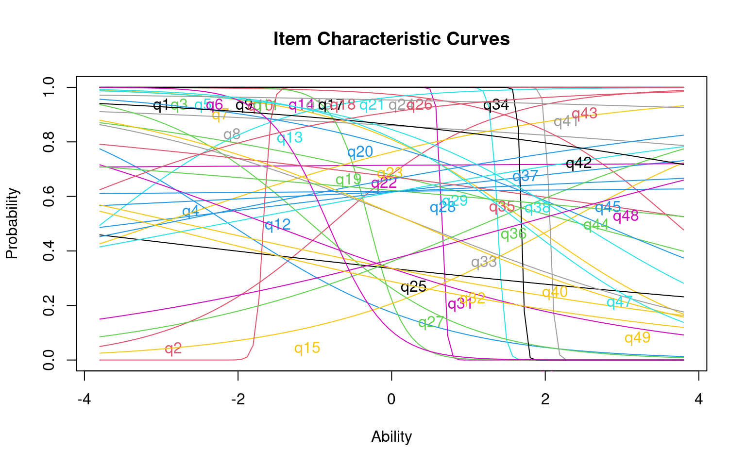
Notice that items vary in their difficulty and discriminibility, and that some are negatively discrimination. It is sort of a mess. This is not unexpected because we have so few participants in this test–there just isn’t enough information to reliably and stably estimate anything. Before we go on, we can look at a few things about how well the model fits:
Item-Fit Statistics and P-values

Call:
ltm(formula = dat ~ z1)

Alternative: Items do not fit the model
Ability Categories: 10

         X^2 Pr(>X^2)
q1    0.0000        1
q2    8.1511   0.4189
q3    0.0000        1
q4    7.6834    0.465
q5    0.1379        1
q6    0.2621        1
q7    9.2744   0.3197
q8    8.7169   0.3667
q9    0.0000        1
q10   4.8496   0.7735
q11   1.5435    0.992
q12   3.4025   0.9066
q13   6.8417   0.5538
q14   0.0000        1
q15   6.0480   0.6419
q16   9.9338   0.2697
q17   0.0000        1
q18 133.4230  <0.0001
q19   7.9250   0.4408
q20   6.6433   0.5756
q21   0.0000        1
q22   7.9145   0.4419
q23  11.6092   0.1695
q24   0.0000        1
q25  14.2920   0.0745
q26   0.0000        1
q27   5.5064   0.7023
q28   9.7243   0.2849
q29   7.9233    0.441
q31   6.2791    0.616
q32   6.0579   0.6407
q33   6.5497   0.5859
q34   0.0000        1
q35   9.1083   0.3332
q36   2.4719    0.963
q37   8.9905   0.3431
q38   7.7650   0.4568
 [ reached 'max' / getOption("max.print") -- omitted 10 rows ]
This gives a ‘fit’ parameter for each question. A few items, like Q18, have bad fit parameters. Looking at the psych::alpha function, it has very low item-whole correlation.
Some items ( q2 q7 q8 q12 q15 q18 q23 q28 q29 q36 q37 q42 q44 q45 ) were negatively correlated with the total scale and
probably should be reversed.
To do this, run the function again with the 'check.keys=TRUE' option
Reliability analysis
Call: psych::alpha(x = dat)

  raw_alpha std.alpha G6(smc) average_r S/N  ase mean    sd median_r
      0.63      0.62     0.6      0.04 1.6 0.11 0.69 0.093    0.038

    95% confidence boundaries
         lower alpha upper
Feldt     0.36  0.63  0.82
Duhachek  0.41  0.63  0.85

 Reliability if an item is dropped:
    raw_alpha std.alpha G6(smc) average_r S/N var.r med.r
q2       0.65      0.64    0.63     0.045 1.8 0.050 0.040
q4       0.63      0.62    0.61     0.042 1.7 0.050 0.037
q5       0.62      0.60    0.58     0.038 1.5 0.049 0.038
q6       0.59      0.58    0.56     0.035 1.4 0.049 0.037
q7       0.60      0.60    0.58     0.037 1.5 0.049 0.037
q8       0.63      0.63    0.61     0.042 1.7 0.050 0.040
q10      0.62      0.61    0.60     0.039 1.6 0.050 0.038
q11      0.62      0.61    0.59     0.040 1.6 0.049 0.038
q12      0.62      0.60    0.60     0.039 1.5 0.050 0.038
q13      0.63      0.62    0.61     0.042 1.6 0.049 0.040
 [ reached 'max' / getOption("max.print") -- omitted 29 rows ]

 Item statistics
     n  raw.r  std.r   r.cor r.drop mean   sd
q2  21 -0.048 -0.093 -0.2498 -0.157 0.67 0.48
q4  21  0.135  0.119  0.0231  0.042 0.19 0.40
q5  21  0.375  0.410  0.3985  0.301 0.86 0.36
q6  21  0.642  0.636  0.6890  0.569 0.67 0.48
q7  21  0.496  0.450  0.4491  0.415 0.76 0.44
q8  21  0.119  0.099 -0.0027  0.037 0.86 0.36
q10 21  0.293  0.303  0.2607  0.246 0.95 0.22
q11 21  0.287  0.280  0.2300  0.177 0.38 0.50
q12 21  0.382  0.346  0.3159  0.279 0.62 0.50
q13 21  0.083  0.147  0.0588  0.033 0.95 0.22
 [ reached 'max' / getOption("max.print") -- omitted 29 rows ]

Non missing response frequency for each item
       0    1 miss
q2  0.33 0.67    0
q4  0.81 0.19    0
q5  0.14 0.86    0
q6  0.33 0.67    0
q7  0.24 0.76    0
q8  0.14 0.86    0
q10 0.05 0.95    0
q11 0.62 0.38    0
q12 0.38 0.62    0
q13 0.05 0.95    0
q15 0.76 0.24    0
q16 0.05 0.95    0
q18 0.05 0.95    0
q19 0.33 0.67    0
q20 0.24 0.76    0
q22 0.29 0.71    0
q23 0.24 0.76    0
q25 0.67 0.33    0
q27 0.71 0.29    0
q28 0.38 0.62    0
q29 0.38 0.62    0
q31 0.67 0.33    0
q32 0.67 0.33    0
q33 0.48 0.52    0
q34 0.10 0.90    0
 [ reached getOption("max.print") -- omitted 14 rows ]
We can look at the person-parameters. These tell us how well each person is described by the model. The tests are like a chi-squared test. We assume that a person of a certain ability should be getting problems easier than they are right, and more difficult than they are wrong. If this assumption is violated for a person, that indicates they violate this model, and are somehow different from the rest of the class which determines the model. Possibly they were cheating so they didn’t get many right but the ones they got right were the most difficult.
Person-Fit Statistics and P-values

Call:
ltm(formula = dat ~ z1)

Alternative: Inconsistent response pattern under the estimated model

  q1 q2 q3 q4 q5 q6 q7 q8 q9 q10 q11 q12 q13 q14 q15 q16 q17 q18 q19 q20 q21
1  1  0  1  0  1  0  0  1  1   1   0   0   1   1   0   1   1   1   1   1   1
  q22 q23 q24 q25 q26 q27 q28 q29 q31 q32 q33 q34 q35 q36 q37 q38 q39 q40 q41
1   1   0   1   1   1   1   0   0   0   1   0   1   0   1   1   0   0   0   1
  q42 q43 q44 q45 q47 q48 q49       L0      Lz Pr(<Lz)
1   1   1   0   0   1   0   0 -22.3816 -1.7917  0.0366
 [ reached 'max' / getOption("max.print") -- omitted 20 rows ]
These are not bad–most people are reasonably-well fit in the model.
The margins() function looks at whether there are
particular parings of items that happen more often than by chance.
Call:
ltm(formula = dat ~ z1)

Fit on the Two-Way Margins

Response: (0,0)
  Item i Item j Obs  Exp (O-E)^2/E
1     13     37   1 0.11      6.86 ***
2      7     28   5 1.72      6.28 ***
3     13     42   1 0.14      5.32 ***

Response: (1,0)
  Item i Item j Obs  Exp (O-E)^2/E
1      7     33   2 0.37      7.24 ***
2     30     33   1 0.15      5.04 ***
3      4     41   2 0.51      4.31 ***

Response: (0,1)
  Item i Item j Obs  Exp (O-E)^2/E
1     16     30   1 0.07     11.81 ***
2      5      7   3 0.88      5.15 ***
3     33     43   2 0.49      4.65 ***

Response: (1,1)
  Item i Item j Obs  Exp (O-E)^2/E
1     30     47   5 2.20      3.55 ***
2      4     15   2 0.71      2.32
3     39     46   7 4.02      2.21

'***' denotes a chi-squared residual greater than 3.5
For example, consider the first line. According to the model, we’d expect 0.11 people to get both 13 and 37 wrong. But the margins show 1 person got them both wrong, which would be unlikely to happen by chance. We can check the table here:
     0  1
  0  1  0
  1  3 17
These might indicate that there are questions that are not independent and so may violate the model assumptions. For 30 and 47, we’d expect only 2.06 people to get them both correct, but 5 did. In these cases, the two questions might be redundant. In other cases, this could capture things like ‘leakage’, where you learn the answer to one question based on another; or exclusive-or choices, where there are two parallel questions with one attractive answer so that people who are guessing are likely to either get them both right or wrong, or are likely to get only one right and the other wrong.
Multiple latent traits
The simple ltm model is essentially logistic regression, but at its core assumes your test measures a single ability dimension. What if your test meaured multiple dimensions that differed systematically and indepedently across people? Usually, you might do a PCA or factor analysis to examine this, but the ltm model will let you test up to two latent traits directly. This should also remind you a bit of how MANOVA works.
As a brief example, here is how we’d do multiple latent traits.
Call:
ltm(formula = dat[, 1:15] ~ z1)

Coefficients:
            Dffclt  Dscrmn
q1   -1.802629e+08   0.000
q2    9.910000e-01  -0.864
q3   -1.802629e+08   0.000
q4    5.842000e+00   0.254
q5   -1.494000e+00   1.581
q6   -6.030000e-01  28.245
q7   -8.320000e-01   2.301
q8   -9.028000e+00   0.198
q9   -1.802629e+08   0.000
q10  -1.449000e+00  12.044
q11   3.520000e-01  27.475
q12   1.140900e+01  -0.043
q13   2.567000e+00  -1.604
q14  -1.802629e+08   0.000
q15  -1.656000e+00  -0.750

Log.Lik: -99.018
Item-Fit Statistics and P-values

Call:
ltm(formula = dat[, 1:15] ~ z1)

Alternative: Items do not fit the model
Ability Categories: 10

        X^2 Pr(>X^2)
q1   0.0000        1
q2  15.4790   0.0505
q3   0.0000        1
q4  13.1159   0.1079
q5   9.8377   0.2766
q6   0.0956        1
q7   5.3522   0.7194
q8   8.1935   0.4148
q9   0.0000        1
q10  1.9348   0.9829
q11  0.0621        1
q12 13.6124   0.0924
q13  5.8759   0.6611
q14  0.0000        1
q15  6.9981   0.5368
Call:
ltm(formula = dat[, 1:15] ~ z1 + z2)

Coefficients:
     (Intercept)       z1        z2
q1        65.566    0.000     0.000
q2         1.236   -0.537     1.942
q3        65.566    0.000     0.000
q4      -121.843  105.913    59.674
q5       185.353  107.015  -142.073
q6        47.280   98.106   -39.255
q7       103.551  147.976    37.214
q8         2.165    0.775     0.896
q9        65.566    0.000     0.000
q10      143.812   93.717   -18.639
q11      -74.365  111.343  -148.643
q12        0.523    0.274     0.552
q13        3.472   -0.503     0.906
q14       65.566    0.000     0.000
q15       -1.578   -0.019     1.505

Log.Lik: -85.347
 Likelihood Ratio Table
           AIC    BIC log.Lik   LRT df p.value
model4a 258.04 289.37  -99.02
model4b 260.69 307.70  -85.35 27.34 15   0.026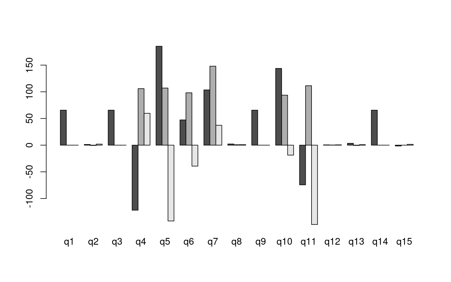
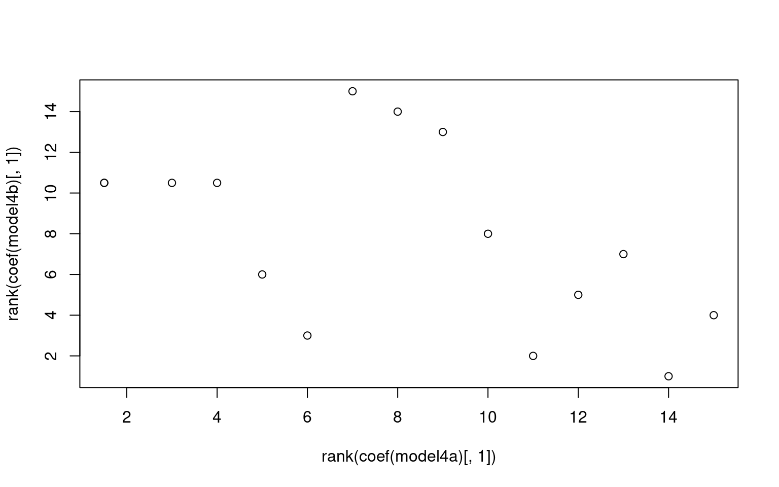
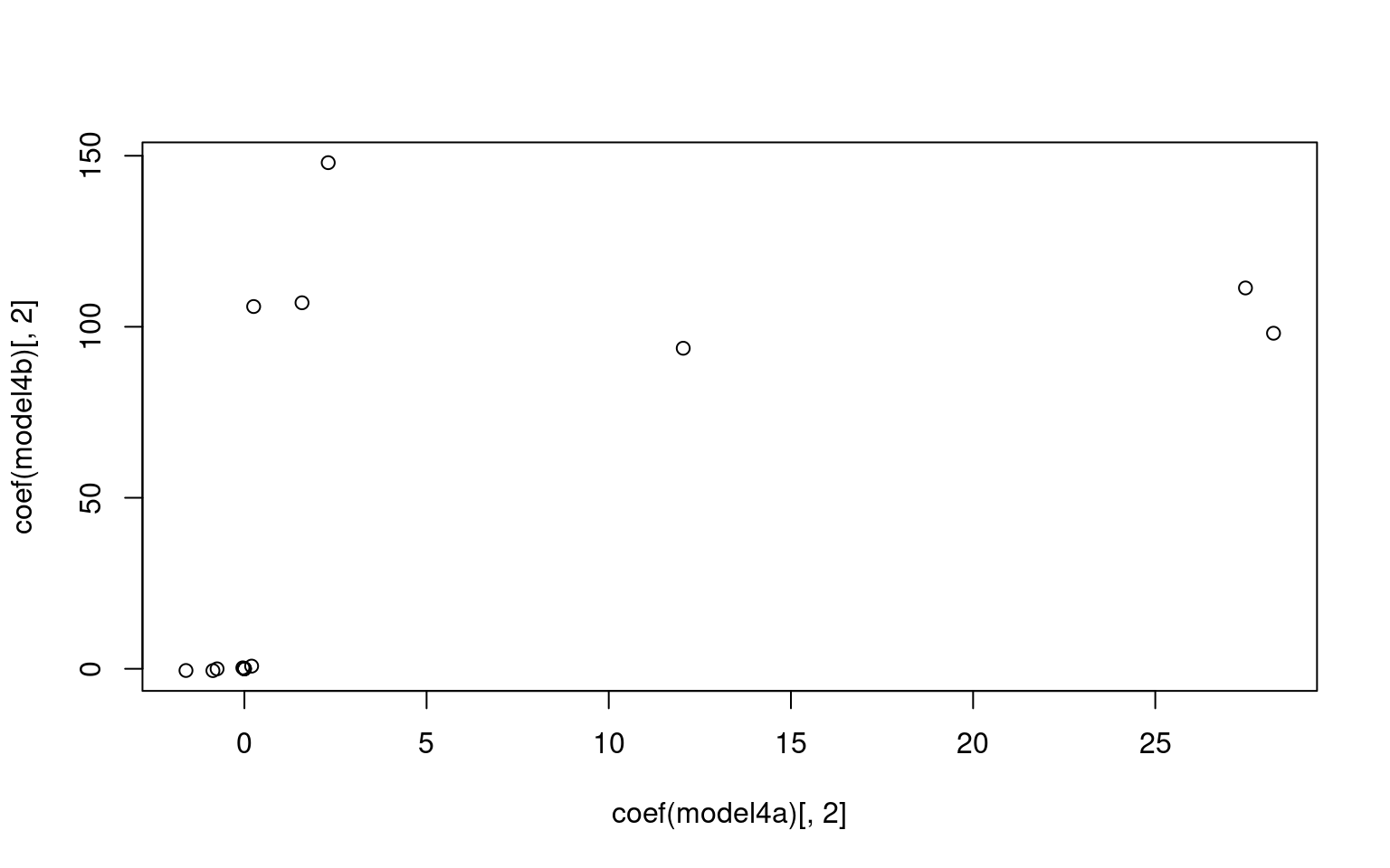
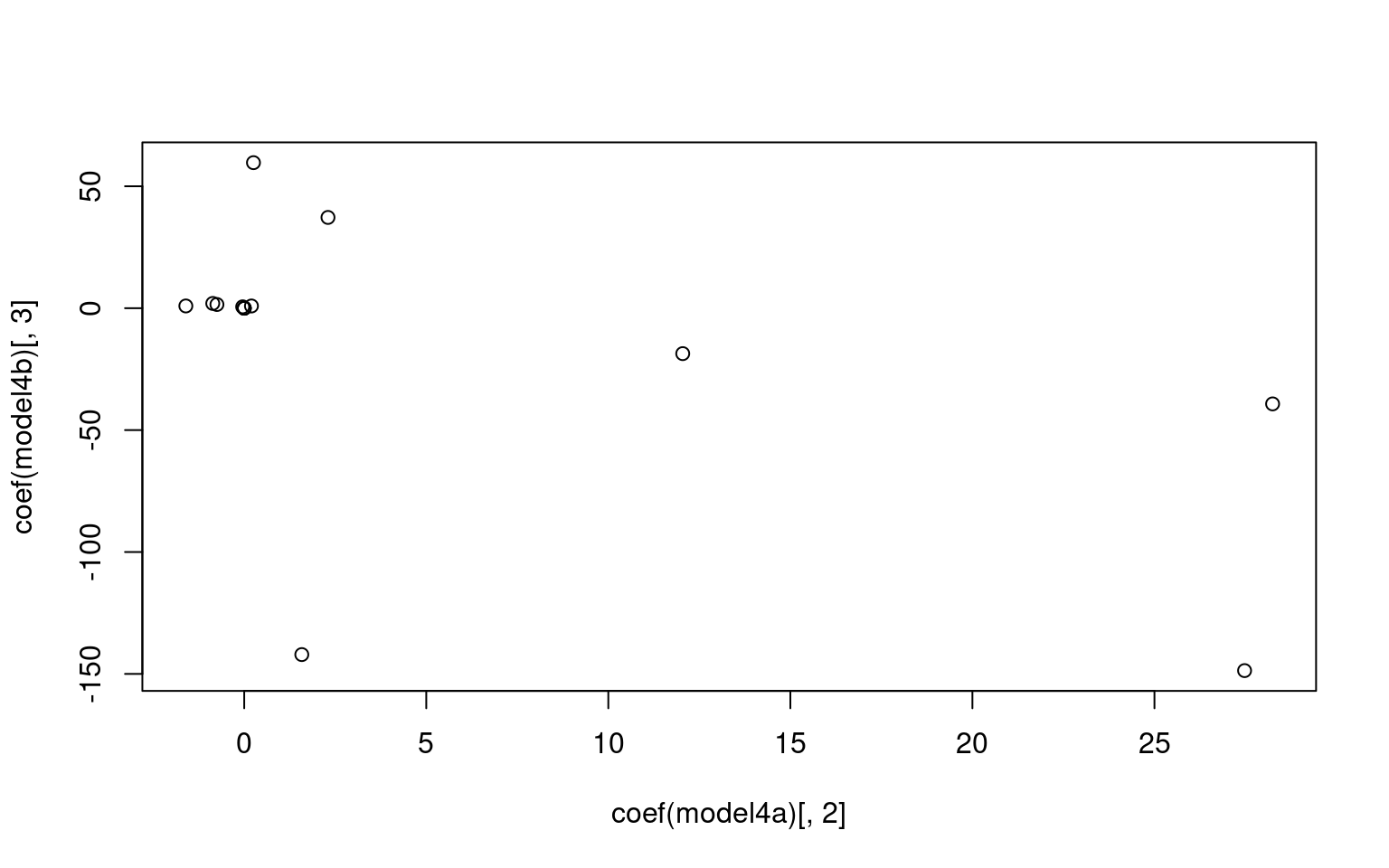
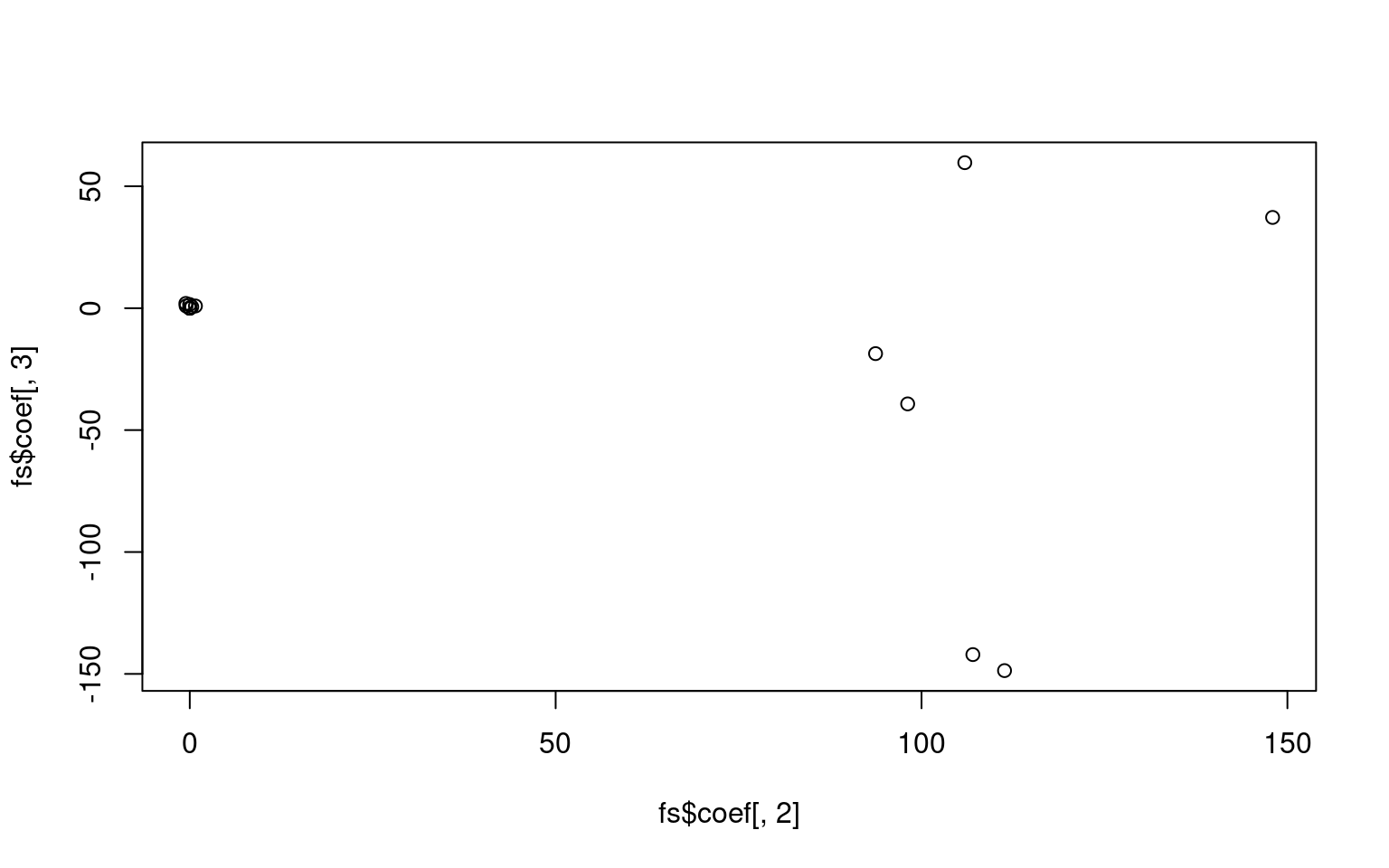 For the z1 only model, we get a difficulty and discriminability
parameter, which is like a mean and variance. For the z1 + z2 model, we
get intercept which is going to be akin to the difficulty parameter, and
z1/z2 represent variance along two principle components. Here, we don’t
see too much similarity across models, but with a larger data set it is
likely we would. It is also likely that z1 or z2 is going to be similar
to the discriminability parameter, but not guaranteed. Here, we see z2
is somewhat correlated with the discriminability
For the z1 only model, we get a difficulty and discriminability
parameter, which is like a mean and variance. For the z1 + z2 model, we
get intercept which is going to be akin to the difficulty parameter, and
z1/z2 represent variance along two principle components. Here, we don’t
see too much similarity across models, but with a larger data set it is
likely we would. It is also likely that z1 or z2 is going to be similar
to the discriminability parameter, but not guaranteed. Here, we see z2
is somewhat correlated with the discriminability
Guessing parameters: the three-parameter model
If you have questions that differ in the ability to get the question right by chance, you might want to incorporate a guessing parameter. These are just the normal ltm model, but bottom out at a lower level that you either estimate or specify. This might be useful if you have a true/false test, where accuracy should be at least 50%, especially if this is mixed with other questions like short answer or multiple choice where guessing accuracy would be lower. In this case, you could fix the parameters based on question type. Otherwise, you might want to estimate them directly–but you would need to be sure you had enough data to get good estimates.
This model is called the three-parameter model (TPM). It incorporates a guessing value, if the chance of getting an answer right is non-zero by guessing.
Call:
tpm(data = dat[, 1:15], type = "latent.trait", max.guessing = 0.5)

Coefficients:
     Gussng         Dffclt   Dscrmn
q1    0.025  -4.775907e+08    0.000
q2    0.054  -9.160000e-01    0.806
q3    0.029  -4.775662e+08    0.000
q4    0.174  -1.884500e+01   -0.200
q5    0.113   1.031000e+00   -3.043
q6    0.014   4.510000e-01  -18.446
q7    0.463   1.230000e-01   -6.073
q8    0.051   2.353800e+01   -0.074
q9    0.032  -4.775418e+08    0.000
q10   0.048   1.513000e+00   -6.885
q11   0.000  -3.800000e-01  -22.118
q12   0.072  -2.603000e+00    0.144
q13   0.048  -1.916000e+00    3.428
q14   0.036  -4.775173e+08    0.000
q15   0.003   1.715000e+00    0.722

Log.Lik: -98.513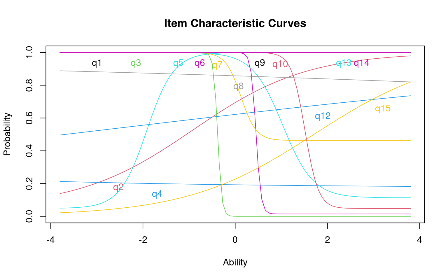 Notice how different items bottom out at different levels.
With a small class, there are a lot of items with negative discriminability. Let’s look at how they work out, by comparing average test score to particular answers:
par(mfrow = c(2, 2))
boxplot(dat$q5, rowMeans(dat), main = "Correct on q5", names = c("Incorrect (3)",
    "correct (18)"))

boxplot(dat$q4, rowMeans(dat), main = "Correct on q4", names = c("Incorrect (1)",
    "correct (20)"))

boxplot(dat$q10, rowMeans(dat), main = "Correct on q10", names = c("Incorrect (3)",
    "correct (18)"))

boxplot(dat$q11, rowMeans(dat), main = "Correct on q11", names = c("Incorrect (13)",
    "correct (8)"))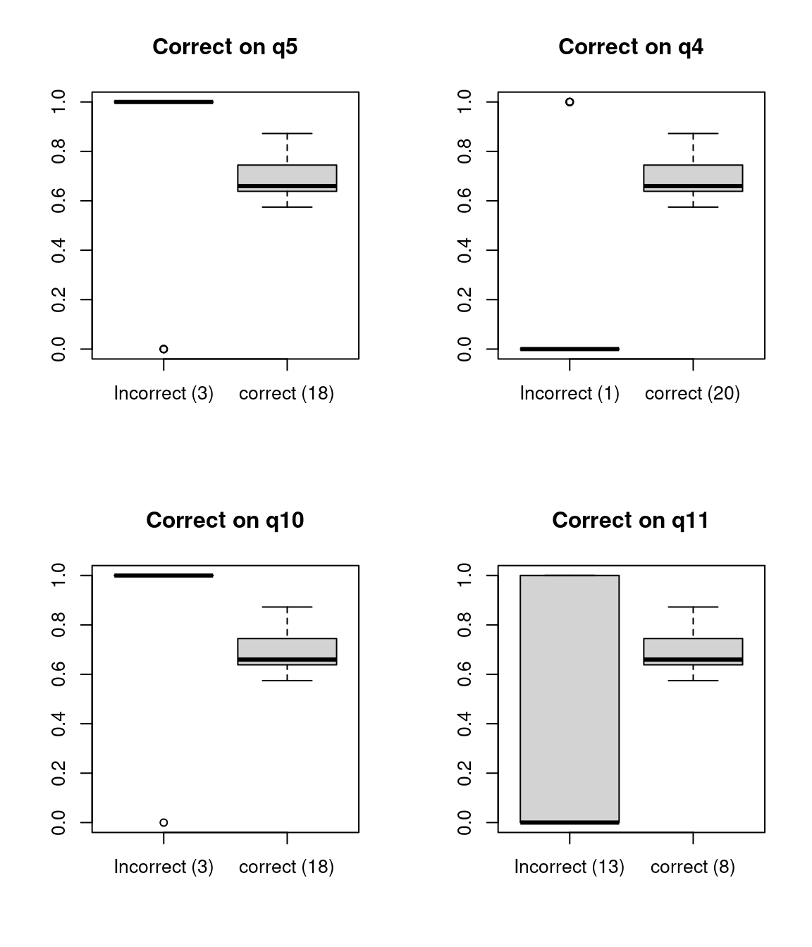
We can see that for some of these, accuracy on the question is negatively correlated with accuracy on the test. For others, there are other strange things, like very small numbers of errors that might make estimation difficult.
Information curves
Each questions can be transformed into an information score, which is the distribution of information implied by the cumulative score. Also, you can plot the characteristic of the entire test:

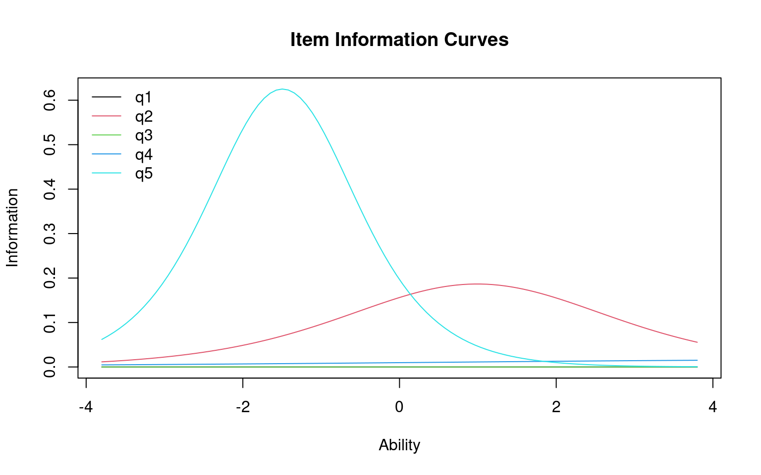
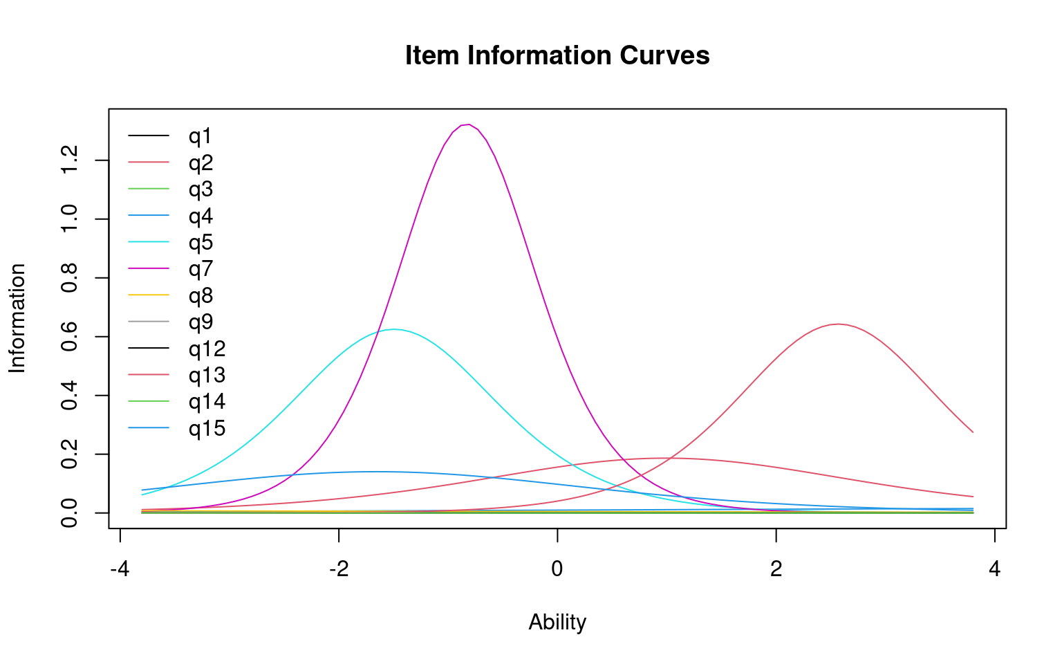 The height of the curve indicates where the most informative ability
level for each question is. A very discriminative question will have a
sharp rise at a specific point, and you would be good at separating
those below from those above.
The height of the curve indicates where the most informative ability
level for each question is. A very discriminative question will have a
sharp rise at a specific point, and you would be good at separating
those below from those above.
Call:
ltm(formula = dat[, c(1, 3, 5, 9, 14)] ~ z1)

Coefficients:
            Dffclt  Dscrmn
q1   -1.321958e+11   0.000
q3   -1.321958e+11   0.000
q5    1.188000e+00  -3.667
q9   -1.321958e+11   0.000
q14  -1.321958e+11   0.000

Log.Lik: -8.612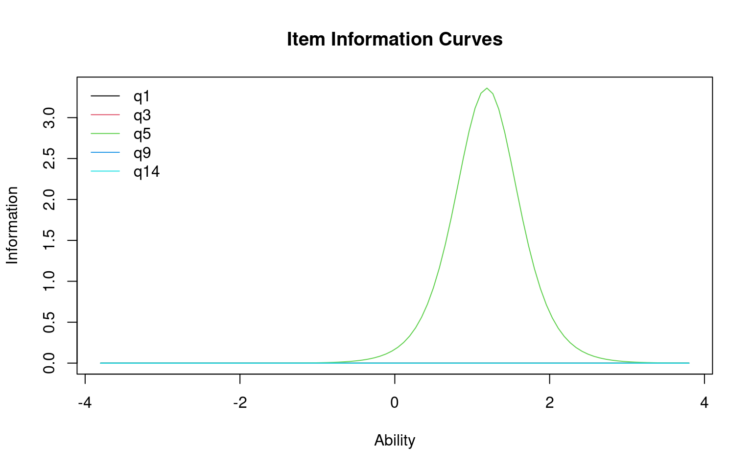
You can specify different items, or items=0 tells you the entire test. This tells you the range of abilities that the test or items will be good at. You can also specify a range to integrate over, to see which range the test is best at discriminating. This can be used to understand whether the test is good at discrimating low-performers (maybe a test for remidial instruction) on high-performers (a test for entrance into a competitive class or program).
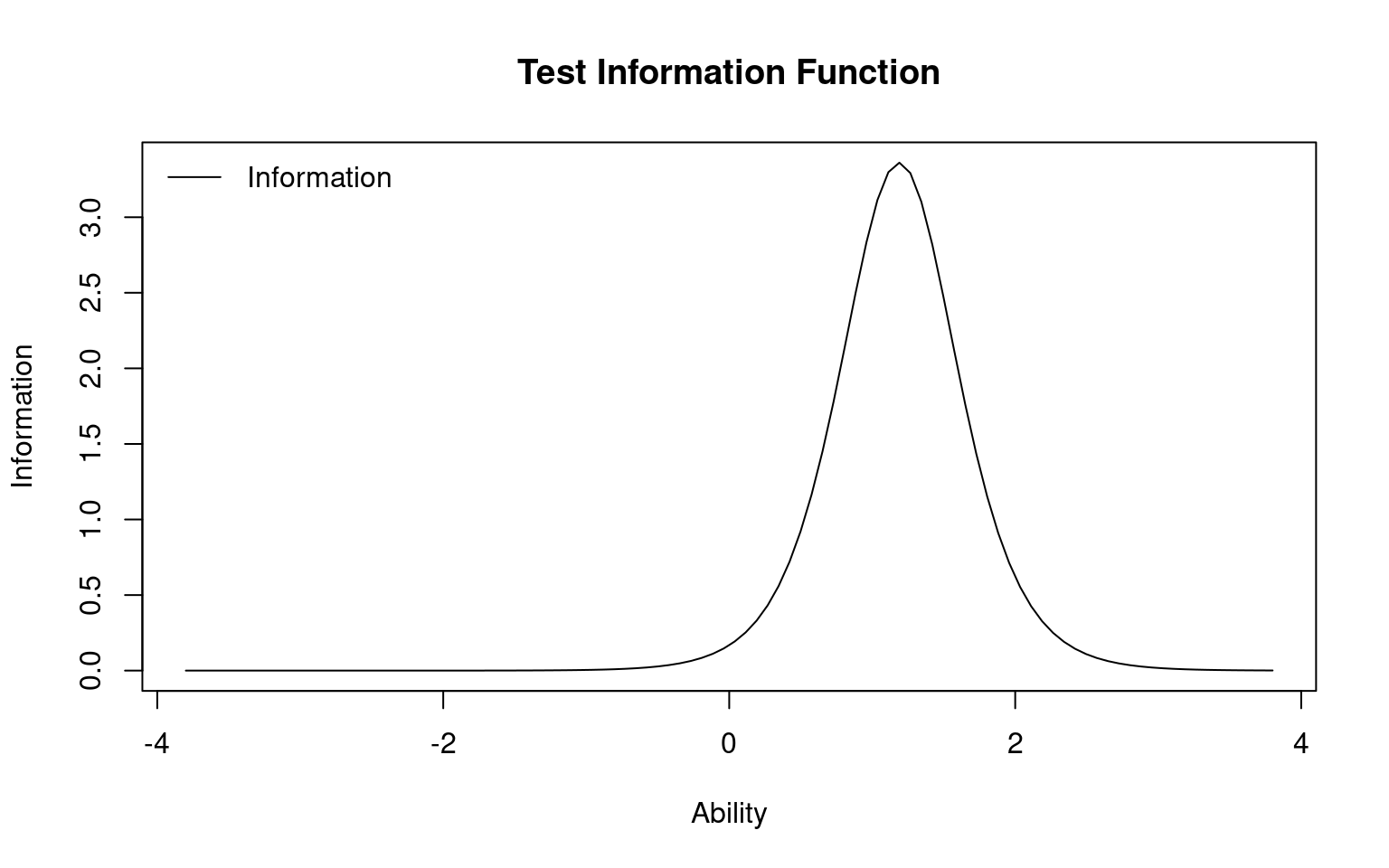
Call:
ltm(formula = dat[, c(1, 3, 5, 9, 14)] ~ z1)

Total Information = 3.67
Information in (-4, 4) = 3.67 (100%)
Based on all the items
Graded response model and partial credit model.
The ltm library provides five models, rasch, ltm, tpm, grm (graded response model-polytomous) and gpcm (general partial credit-polytomous). These last two are appropriate for rank-order and categorical responses, and might be useful for evaluating personality scales.
The basic assumptions of IRT is that you have a binary outcome (correct or incorrect). But it could be interesting to do an IRT-like analysis for non-binary responses. If you have a set of likert-scale responses, where they are all coded in the same direction, and they each independently give support for some construct, you can use a graded response model. This might be useful for personality data, for example. Let’s consider measures from the big five personality questionnaire we have examined in the past.
A related model in the ltm package is the graded partial credit model (gpcm). This would allow you to place an ordinal scale on correctness, and do an IRT analysis. Maybe in a short answer response, you score full credit for one response, and partial credit for another. We won’t cover this model here, but it has some similarity to the GRM.
To examine the GRM, Let’s obtain just the introversion/extraversion values, and reverse code so they are all in the same direction. for convenience, I’ll also remove any values that are NA.
big5 <- read.csv("bigfive.csv")
qtype <- c("E", "A", "C", "N", "O", "E", "A", "C", "N", "O", "E", "A", "C", "N",
    "O", "E", "A", "C", "N", "O", "E", "A", "C", "N", "O", "E", "A", "C", "N", "O",
    "E", "A", "C", "N", "O", "E", "A", "C", "N", "O", "O", "A", "C", "O")
valence <- c(1, -1, 1, 1, 1, -1, 1, -1, -1, 1, 1, -1, 1, 1, 1, 1, 1, -1, 1, 1, -1,
    1, -1, -1, 1, 1, -1, 1, 1, 1, -1, 1, 1, -1, -1, 1, -1, 1, 1, 1, -1, 1, -1, 1)
## reverse code
for (i in 2:ncol(big5)) {
    if (valence[i - 1] == -1) {
        big5[, i] <- 6 - big5[, i]
    }
}
ei <- big5[, c(T, qtype == "E")]
ei <- ei[!is.na(rowSums(ei)), ]
Now, the graded response model in ltm (grm) will do a irt-like analysis, treating these as ordinal values. You can use a constrained or unconstrained model–the constrained model fits an equal discriminability across all questions. Because we have a lot of data, this model takes a while to fit.
Call:
grm(data = ei[, -1], constrained = TRUE)

Coefficients:
     Extrmt1  Extrmt2  Extrmt3  Extrmt4  Dscrmn
Q1    -2.210   -0.924   -0.150    1.233   1.684
Q6    -1.531    0.123    0.838    2.007   1.684
Q11   -2.729   -1.194   -0.359    1.068   1.684
Q16   -2.853   -1.410   -0.370    1.061   1.684
Q21   -1.356    0.100    0.702    1.863   1.684
Q26   -2.003   -0.861   -0.116    1.360   1.684
Q31   -1.389    0.368    0.865    1.971   1.684
Q36   -2.579   -1.099   -0.468    0.984   1.684

Log.Lik: -10583.71
Call:
grm(data = ei[, -1], constrained = TRUE)
Model Summary:
log.Lik AIC BIC
-10583.71 21233.41 21395.7
Coefficients:
$Q1
value
Extrmt1 -2.210
Extrmt2 -0.924
Extrmt3 -0.150
Extrmt4 1.233
Dscrmn 1.684
$Q6
value
Extrmt1 -1.531
Extrmt2 0.123
Extrmt3 0.838
Extrmt4 2.007
Dscrmn 1.684
$Q11
value
Extrmt1 -2.729
Extrmt2 -1.194
Extrmt3 -0.359
Extrmt4 1.068
Dscrmn 1.684
$Q16
value
Extrmt1 -2.853
Extrmt2 -1.410
Extrmt3 -0.370
Extrmt4 1.061
Dscrmn 1.684
$Q21
value
Extrmt1 -1.356
Extrmt2 0.100
Extrmt3 0.702
Extrmt4 1.863
Dscrmn 1.684
$Q26
value
Extrmt1 -2.003
Extrmt2 -0.861
Extrmt3 -0.116
Extrmt4 1.360
Dscrmn 1.684
$Q31
value
Extrmt1 -1.389
Extrmt2 0.368
Extrmt3 0.865
Extrmt4 1.971
Dscrmn 1.684
$Q36
value
Extrmt1 -2.579
Extrmt2 -1.099
Extrmt3 -0.468
Extrmt4 0.984
Dscrmn 1.684
Integration:
method: Gauss-Hermite
quadrature points: 21
Optimization:
Convergence: 0
max(|grad|): 0.0094
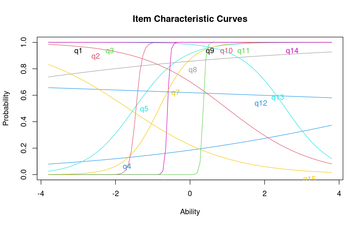
quasi-Newton: BFGS We can see that each question is modeled with its own IRT-like model. There are five levels here, and four transitions between levels, which are modeled as sort of difficulty parameters for each transition between items.
Plotting each question gives us another look
par(mfrow = c(4, 2))
plot(g1, items = 1)
plot(g1, items = 2)
plot(g1, items = 3)
plot(g1, items = 4)
plot(g1, items = 5)
plot(g1, items = 6)
plot(g1, items = 7)
plot(g1, items = 8)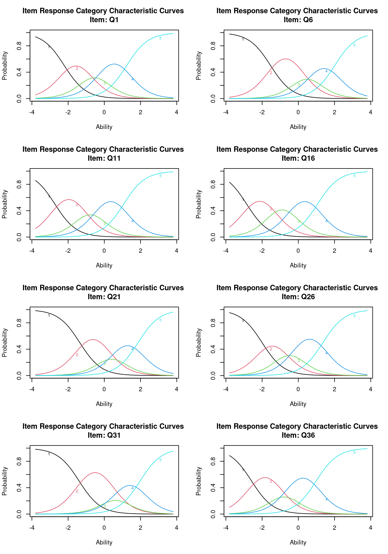 The margins() function works here as well. We can see that there are a
couple that violate the two-way independence (q1-q21; q6-q21, etc.)
The margins() function works here as well. We can see that there are a
couple that violate the two-way independence (q1-q21; q6-q21, etc.)
Call:
grm(data = ei[, -1], constrained = TRUE)

Fit on the Two-Way Margins

    Q1  Q6     Q11    Q16    Q21    Q26    Q31    Q36
Q1  -    25.82  50.38  37.85 102.57  67.00  82.91  72.89
Q6      -       44.89  50.86 124.08  73.31  44.03  37.03
Q11            -       96.73  55.00  76.17  84.33  45.93
Q16            ***    -       55.38  51.31  65.46  52.74
Q21 *** ***                  -       53.24  74.63  29.73
Q26                                 -       62.84  37.69
Q31                                        -       34.28
Q36                                               -

'***' denotes pairs of items with lack-of-fit
Let’s fit this unconstrained:
Call:
grm(data = ei[, -1], constrained = FALSE)

Coefficients:
     Extrmt1  Extrmt2  Extrmt3  Extrmt4  Dscrmn
Q1    -1.927   -0.814   -0.137    1.076   2.215
Q6    -1.531    0.121    0.838    2.010   1.682
Q11   -2.916   -1.276   -0.384    1.140   1.509
Q16   -2.766   -1.370   -0.363    1.029   1.773
Q21   -1.269    0.090    0.655    1.742   1.907
Q26   -2.549   -1.088   -0.137    1.732   1.164
Q31   -1.511    0.395    0.939    2.150   1.459
Q36   -2.302   -0.988   -0.426    0.877   2.090

Log.Lik: -10539.91
Call:
grm(data = ei[, -1], constrained = FALSE)

Model Summary:
   log.Lik      AIC      BIC
 -10539.91 21159.82 21356.53

Coefficients:
$Q1
         value
Extrmt1 -1.927
Extrmt2 -0.814
Extrmt3 -0.137
Extrmt4  1.076
Dscrmn   2.215

$Q6
         value
Extrmt1 -1.531
Extrmt2  0.121
Extrmt3  0.838
Extrmt4  2.010
Dscrmn   1.682

$Q11
         value
Extrmt1 -2.916
Extrmt2 -1.276
Extrmt3 -0.384
Extrmt4  1.140
Dscrmn   1.509

$Q16
         value
Extrmt1 -2.766
Extrmt2 -1.370
Extrmt3 -0.363
Extrmt4  1.029
Dscrmn   1.773

$Q21
         value
Extrmt1 -1.269
Extrmt2  0.090
Extrmt3  0.655
Extrmt4  1.742
Dscrmn   1.907

$Q26
         value
Extrmt1 -2.549
Extrmt2 -1.088
Extrmt3 -0.137
Extrmt4  1.732
Dscrmn   1.164

$Q31
         value
Extrmt1 -1.511
Extrmt2  0.395
Extrmt3  0.939
Extrmt4  2.150
Dscrmn   1.459

$Q36
         value
Extrmt1 -2.302
Extrmt2 -0.988
Extrmt3 -0.426
Extrmt4  0.877
Dscrmn   2.090


Integration:
method: Gauss-Hermite
quadrature points: 21

Optimization:
Convergence: 0
max(|grad|): 0.0097
quasi-Newton: BFGS par(mfrow = c(4, 2))
plot(g2, items = 1)
plot(g2, items = 2)
plot(g2, items = 3)
plot(g2, items = 4)
plot(g2, items = 5)
plot(g2, items = 6)
plot(g2, items = 7)
plot(g2, items = 8)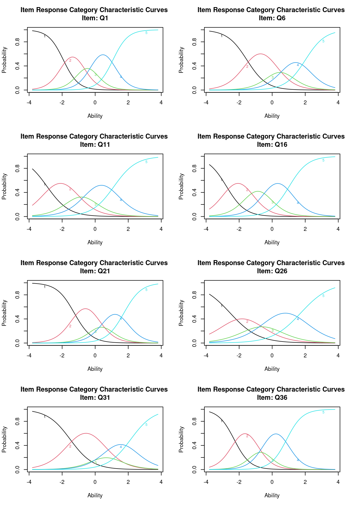
For this model, we might consider the midpoint transition (extrm2) is the ‘center’ of the question. We can see that Q36 and Q26 are low, while Q21 and Q31 are high. We might also use this to infer that a 4 on Q36 is about equivalent to a 3 on Q21.
Discussion and Conclusions about the IRT model
The basic IRT/Rasch model is ubiquitous in areas of testing and measurement. It is helpful for designing tests that are maximally predictive using the smallest number of questions. It does not completely replace more traditional psychometric approaches, but augments them so that you can design smaller more effective tests, and is an important tool that both educators and researchers are typically not aware of, even if it can be helpful.
Additional data
For practice, the resource folder includes a worked example of IRT on a crossword-puzzle experiment (crossword.csv), and a data set quizgrades.csv with 49 students answers on 13 problems.
Additional resources
- There are special-purpose standalone software packages many people use for IRT style models. SPSS recommends that you use an R package via their R connector.
- The
mirtlibrary estimates IRT models. It also has a companion mirtCat and ggmirt library for using it in other contexts. (ggmirt is not in the CRAN and needs to be downloaded). A number of people have shown how to use ggplot with mirt on various blogs. MIRT looks like it can use syntax from some commonly IRT system, and you need to use R to program that other system via a text string, but blogs appear to show simple ways to apply it as well. - The
irtlibrary has objects for representing testbeds and items in a computerized adaptive testing framework, but I’m not sure if it can estimate parameters directly from data. It looks more useful for driving an adaptive test or simulating tests. - Other packages noted by Chalmers, the developer of mirt, include eRm, MCMCpack, and he notes that mirt was the only one to include confirmatory item factor analysis methods, at least in 2012.