Classification: LDA and QDA Approaches
Classification and Categorization
General regression approaches we have used so far have typically had the goal of modeling how a dependent variable (usually continuous, but in the case of logistic regression, binary, or with multinomial regression multiple levels) is predicted by a set of independent variables or predictor variables. The goal of building a regression models often prediction and hypothesis testing. Generally, we are seeking to create an understandable model of the process that we can interpret and make inferences from.
Many times, we might care less about making a numerical prediction, and more about classifying into categories to be able to take action, based on the same measurable properties. This is very similar to the goals of logistic regression, but in logistic regression we are modeling the probability of a binary category, whereas in classification we just care about which category is most likely, and may not really care how probable that category is. Furthermore, logistic regression models the conditional probability of a category given the predictor variables, so it does not really matter if your two categories occur roughly equally or not. But if you know that 90% of cases are of one type, you might use a different criterion for making your classification if you want to maximize the number of correct responses. Classification methods would typically want to consider the overall base rate as well as the relative influence of different factors, in order to maximize the probability of getting the right prediction. Typically, for classification approaches, we need to select a criterion or cut-off of some sort to make a decision–hopefully one that will give the greatest chance of getting a new classification right.
There are many applications for classification, and recently the work on this has migrated from statisticians to computer scientists and specialists in machine classification, machine learning, and artificial intelligence. The goals of classification differ somewhat from approaches like logistic regression and MANOVA. For example, either approach could be used as a tool to help diagnose a disease. A logistic regression would produce the odds that a person has a disease, whereas the a machine classification might be used to determine whether a disease is present–perhaps with some margin of error. A regression might be used to determine the likelihood a company’s will declare bankruptcy, while a classification might be used to identify a set of ‘at-risk’ companies. Overall, these are very similar goals, and although there are many different approaches to achieve this, the solutions can end up looking very similar. Importantly, regression-style models are usually done to test scientific hypotheses, whereas classification models are typically used to make predictions.
Some of the terminology tends to differ across these two approaches. A regression approach might discuss variables, fitting, and inference; a classification might call these features, learning, and cross-validation. There are some aspects of applying regression models and classification models that have similar goals, but different methods. For example, in regression modeling, we often use the ANOVA, analysis of deviance, or a criterion such as AIC to compare models and determine whether a predictor should be used. In classification, the ultimate criterion is often classification accuracy, and a huge aspect of ‘machine learning’ is selecting and removing features to use in a model. In general, the attitude for regression models is typically interpretability, leading to small models with comprehensible measures. Oftentimes, classification approaches might start with hundreds or thousands of features, and combination rules and decision rules might be very abstract and difficult to comprehend. Furthermore, classification is more likely to use separate data sets or cross-validation to do variable selection (feature learning). Regression is more likely to use AIC or BIC methods to select variables on the whole data set.
Classification as Logistic Regression
Logistic regression provides a method for making a prediction about the binary classification of something based on a set of predictors.
In the following data set, we asked participants to judge whether concepts were related. Some of the concepts were engineering terms; others were psychology terms. We tested both engineering and psychology students, and we wanted to know if we could tell them apart based on the speed and accuracy of their responses. Terms were classified into different bins, with e=engineering, p=psychology, r=related, and u=unrelated.
## The following just builds the data set.  ee are eng-eng terms; p-p are
## psych-psych-terms; ep are eng-psych pairs. Colums are the accuracy and mean
## time to make a decision about each kind of word pair.
library(dplyr)

data.raw <- read.csv("samediff-pooled.csv")
data <- dplyr::filter(data.raw, cond %in% c("eerc", "eer", "eeu", "ep", "ppr", "ppu"))


stim <- c(as.character(data$word1), as.character(data$word2))
acc <- c(data$corr, data$corr)
rt <- c(data$rt, data$rt)
sub <- c(data$subnum, data$subnum)
data$pairs <- paste(data$word1, data$word2, sep = "-")

dat.corr <- as.data.frame(tapply(data$corr, list(sub = data$sub, type = factor(data$cond)),
    mean))
dat.rt <- as.data.frame(tapply(data$rt, list(sub = data$sub, type = factor(data$cond)),
    function(x) {
        exp(mean(log(x), na.rm = T))
    }))

dat.joint <- cbind(dat.corr, dat.rt)

survey <- read.csv("survey.csv")
surv2 <- data.frame(sub = survey$subnum, eng = survey$engineering)

joint <- data.frame(eng = surv2$eng, dat.joint)
joint[1:5, ]
eng eer eeu ep ppr ppu eer.1 eeu.1
11 1 0.0000000 1.0000000 0.9166667 1.0000000 0.3333333 3067.054 3456.719
12 1 1.0000000 0.3333333 0.7500000 0.6666667 0.3333333 4802.485 3232.388
13 1 1.0000000 0.3333333 0.8333333 1.0000000 0.6666667 3829.248 2910.454
22 1 0.6666667 0.6666667 0.8333333 1.0000000 1.0000000 5319.195 5402.452
31 1 0.3333333 1.0000000 0.7500000 1.0000000 0.6666667 7986.328 4164.368
ep.1 ppr.1 ppu.1
11 4226.315 7401.313 2964.913
12 4439.391 2307.532 4472.440
13 2703.639 3059.160 2811.498
22 5365.715 5082.285 6943.674
31 7351.413 1057.707 4957.271Let’s start with a logistic regression.
Call:
glm(formula = eng ~ ., family = binomial, data = joint)

Deviance Residuals:
     Min        1Q    Median        3Q       Max
-1.65694  -1.07432  -0.08598   1.09348   1.76901

Coefficients:
              Estimate Std. Error z value Pr(>|z|)
(Intercept) -3.322e+00  2.018e+00  -1.646   0.0997 .
eer          2.279e-02  9.498e-01   0.024   0.9809
eeu          6.761e-01  8.583e-01   0.788   0.4309
ep           9.017e-01  1.916e+00   0.471   0.6380
ppr          3.123e-01  9.844e-01   0.317   0.7510
ppu          1.564e+00  1.043e+00   1.499   0.1337
eer.1       -3.658e-05  2.387e-04  -0.153   0.8782
eeu.1       -1.627e-04  2.979e-04  -0.546   0.5849
ep.1         3.758e-04  3.804e-04   0.988   0.3232
ppr.1       -1.092e-04  2.485e-04  -0.439   0.6605
ppu.1        2.380e-04  2.761e-04   0.862   0.3886
---
Signif. codes:  0 '***' 0.001 '**' 0.01 '*' 0.05 '.' 0.1 ' ' 1

(Dispersion parameter for binomial family taken to be 1)

    Null deviance: 105.36  on 75  degrees of freedom
Residual deviance:  97.54  on 65  degrees of freedom
AIC: 119.54

Number of Fisher Scoring iterations: 4
The residual deviance is a bit large so we might consider a quasi-binomial. We can see that none of the predictors are statistically significant, but nevertheless we can make a prediction about the log-odds of each person being an engineer, and compare it to their actual major:
         0  1
  FALSE 26 14
  TRUE  12 24
This is not bad–about 2/3 correct in each category. Maybe there is a better place to put the criterion. This could be true if we had mostly engineers or mostly psychologists.
[1] 48[1] 50[1] 50[1] 50[1] 47[1] 40If we looked at just the first 50 participants, the best criterion is different:
[1] 35[1] 36[1] 31[1] 29[1] 23[1] 19Here, a criterion of -.25 gives us better classification performance. This is just a consequence of base rate, because more engineers were stored in the first half of the data file. This is OK, but a bit worrisome. None of the predictors were significant, so we might have gotten here just by chance. We might be over-fitting the data. In regression, we’d do inferential test or information criteria to identify which variables to use. Later, we’ll see how this is done for machine classification.
Basics of Machine Classification
We can see how logistic regression can be used as a classifier, as long as we can determine a reasonable criterion. Prior to the widespread use of logistic regression (which requires maximum-likelihood estimation and computerized approaches), various approaches to classification were developed that use simplified models. One traditional model assumes that two groups have multivariate normal distributions with equal variance. In the figure below, we see two such 2-dimensional distributions, with a line drawn between the centers of each, and contours showing the basic data.
library(ggplot2)
set.seed(100)
n <- 500
class <- rep(c("A", "B"), each = n)
x <- rnorm(n * 2, mean = rep(c(3, 4), each = n))
y <- rnorm(n * 2, mean = rep(c(2.5, 1.5), each = n))
ggplot(data.frame(class, y, x), aes(x = x, y = y, colour = class)) + geom_point(size = 1.5) +
    geom_density_2d() + geom_segment(x = -1, y = 6.5, xend = 7, yend = -1.5, col = "grey60",
    lwd = 1.2) + geom_segment(x = 3, y = 2.5, xend = 4, yend = 1.5, col = "black",
    lwd = 1.2) + geom_segment(x = 1.5, y = 0, xend = 5.5, yend = 4, col = "darkgreen") +
    coord_fixed(ratio = 1, xlim = c(0, 6), ylim = c(0, 6)) + theme_bw() + scale_color_manual(values = c("orange",
    "navy"))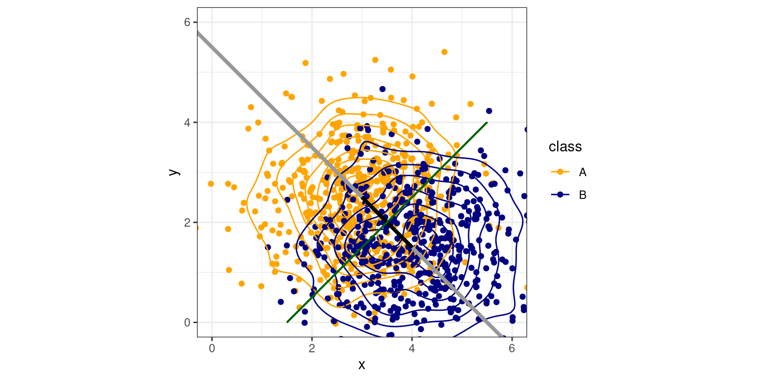
Under our assumptions, if we draw a line between the centers and extend it out (the grey line), we can project any points onto this line (i.e., the closest point on the line to each point). We could use position along this line to predict category membership in a regression or logistic regression–and this is essentially what regression does. This mapping from input variables to a single function is called the discriminant function, and is equivalent to the weighted sum of values by coefficients in regular regression. Now, if we want to classify any observation, we just need to determine which case is more likely. Given the assumptions of equal variance and normality, this can be shown to be a single criterion that maximizes our chances of being correct. In this case, that corresponds to where the green line intersects the black line, and if we move back to the original data, the entire green line is a good rule discriminating the two groups.
Under these assumptions, there are a number of approaches that can be used. In fact, MANOVA is somewhat similar, but framing the model backwards. The most common approach used is referred to as linear discriminant analysis (LDA), or sometimes multivariate discrimination analysis (MDA). The assumptions of this approach are a bit stronger than regression (requiring normal input predictors and equal variances). If these assumptions hold or we can transform them so they work, we can get improved classification results over other methods. In practice, the methods are likely to be almost equivalent to logistic regression.
Linear discriminant analysis
Using the fake data from the figure, we can fit an lda model, using the MASS library, using syntax that looks a lot like lm:
Call:
lda(as.factor(class) ~ x + y)

Prior probabilities of groups:
  A   B
0.5 0.5

Group means:
         x        y
A 2.962393 2.488608
B 4.071218 1.519686

Coefficients of linear discriminants:
         LD1
x  0.7198942
y -0.6940647
We can see that the simple LDA finds the mean of group A and B along the two measured dimensions, and then reports ‘coefficients of linear discriminants’. This is the direction in XY space that best discriminates the two groups. If we could map each observation onto this line, we can easily make a decision that optimally classifies the two groups. We can simply multiply each observed variable by the coefficient to get a sum value, which is the value used to discriminate the two classes, once an optimal threshold is chosen. You can see that if you do predict() on a model, the $class tells you predicted class, and $x tells you the exact values we calculated in LD1.
ldout <- x * 0.71989 + y * (-0.69406)
p <- predict(model0)

plot(p$x, ldout, col = p$class)
abline(0, 1)
grid()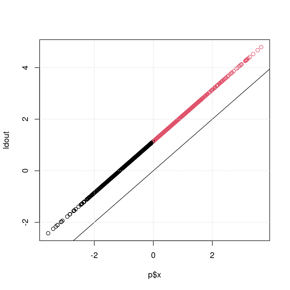
This is a bit clearer if we visualize it, which we can do via the klaR library, which has a number of classification schemes available, including a number of visualization methods. Let’s look at a ‘partimat’ plot:
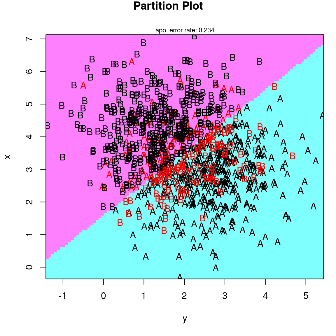
partimat(as.factor(class) ~ x + y, method = "lda", plot.matrix = TRUE, imageplot = FALSE) # takes some time ...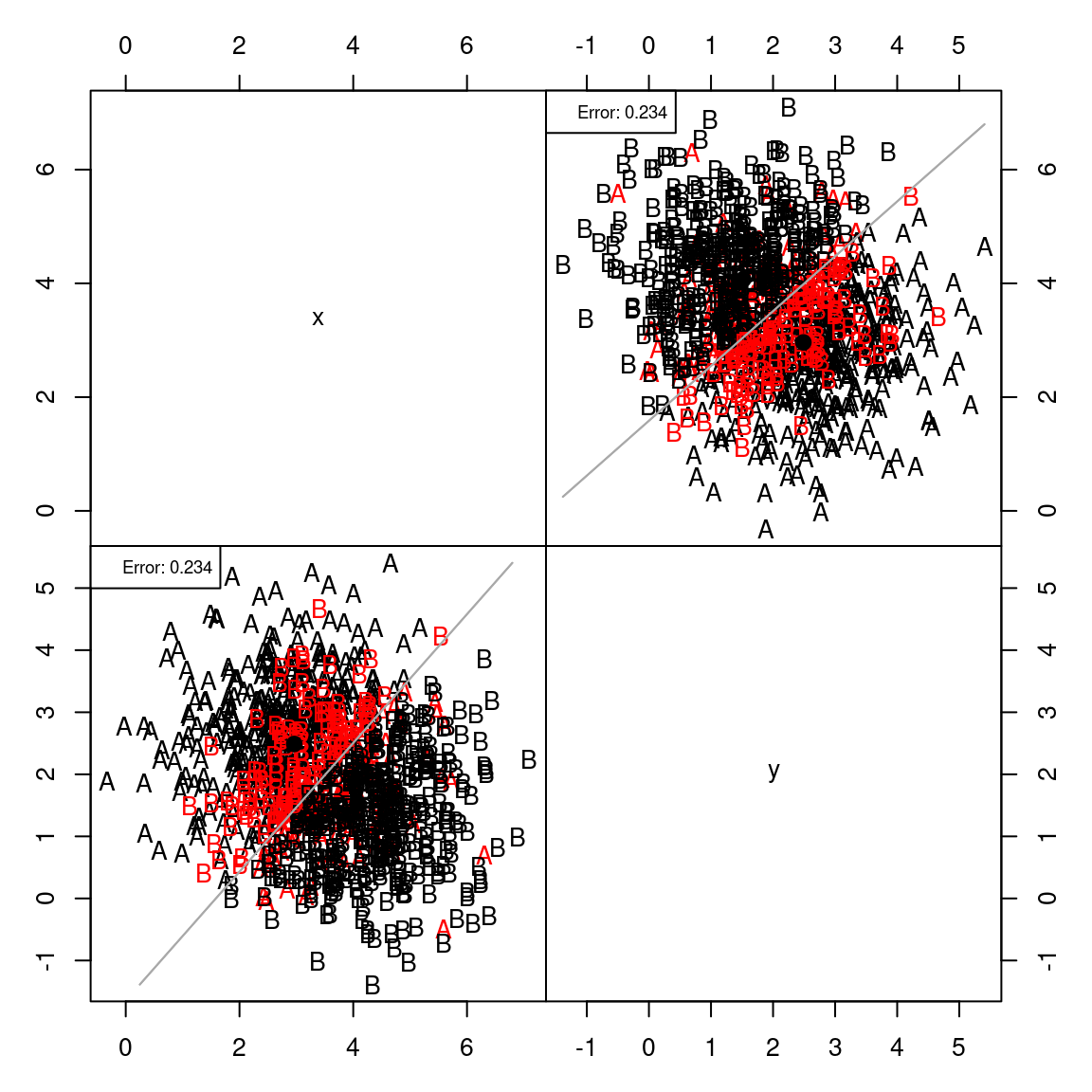
If you think about the line connecting the centers of the two groups, it goes from the upper left to lower right. This direction can be defined by a vector: (.71, -.69), which is a slope of around -1. The red line in the figure shows the decision criterion that best separates the two groups.
Let’s look at the engineering data set, which has more than two predictors
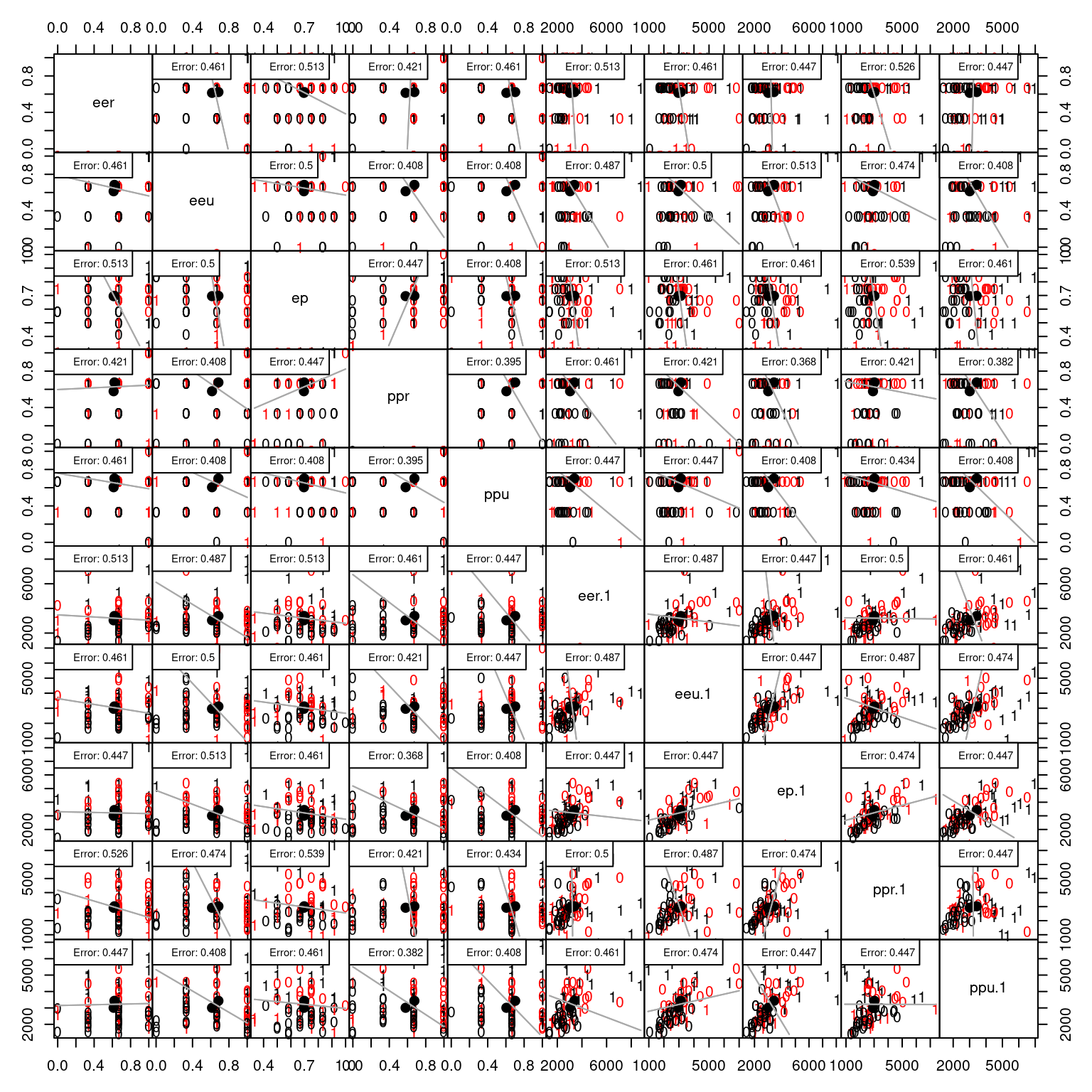
This shows the classification along each pair of dimensions.
Call:
lda(eng ~ ., data = joint)

Prior probabilities of groups:
  0   1
0.5 0.5

Group means:
        eer       eeu        ep       ppr       ppu    eer.1    eeu.1     ep.1
0 0.6140351 0.6140351 0.6951754 0.5789474 0.6052632 3038.008 2962.742 3005.707
1 0.6228070 0.6842105 0.6973684 0.6754386 0.7017544 3387.195 3120.454 3428.785
     ppr.1    ppu.1
0 2921.188 3007.688
1 3024.660 3432.817

Coefficients of linear discriminants:
                LD1
eer    3.672284e-02
eeu    9.989394e-01
ep     1.295582e+00
ppr    4.695055e-01
ppu    2.385932e+00
eer.1 -5.396259e-05
eeu.1 -2.316937e-04
ep.1   4.827826e-04
ppr.1 -1.456996e-04
ppu.1  3.812870e-04
If we look at group means and the coefficients, we can see that a few of the measures differ substantially between the two groups, but not all. The largest coefficients typically map onto the dimensions with the greatest difference between groups.
Predicting class from an LDA model
We can use predict to predict the values of the fitted
data, and then compare these to the true values. The function
confusion in DAAG provides nicely-formatted
output. If we just want to know how many we got correct, we can look at
the diagonal of the table.
$class
 [1] 0 1 0 1 1 0 1 0 1 1 0 0 1 0 1 0 1 1 1 0 0 1 1 1 0 1 0 1 0 1 0 0 0 0 1 1 1 0
[39] 1 0 0 1 0 1 0 0 1 1 0 1 0 0 1 1 1 1 1 0 1 0 0 0 0 1 0 0 0 0 0 1 1 0 0 0 0 0
Levels: 0 1

$posterior
            0         1
11  0.5512784 0.4487216
12  0.4907813 0.5092187
13  0.5540551 0.4459449
22  0.1502546 0.8497454
31  0.1237940 0.8762060
32  0.6055351 0.3944649
33  0.4234531 0.5765469
41  0.6275495 0.3724505
51  0.1367011 0.8632989
52  0.4797138 0.5202862
61  0.5544694 0.4455306
62  0.6745057 0.3254943
63  0.4469692 0.5530308
64  0.6752190 0.3247810
71  0.3398060 0.6601940
81  0.5468117 0.4531883
101 0.4014884 0.5985116
102 0.3694719 0.6305281
104 0.3822059 0.6177941
201 0.8183543 0.1816457
202 0.5981471 0.4018529
203 0.3306295 0.6693705
301 0.4570754 0.5429246
302 0.4452991 0.5547009
303 0.6392452 0.3607548
304 0.2763718 0.7236282
401 0.5196067 0.4803933
402 0.4912082 0.5087918
501 0.5067966 0.4932034
502 0.4105879 0.5894121
503 0.6803426 0.3196574
504 0.5564842 0.4435158
505 0.5814196 0.4185804
507 0.6919807 0.3080193
508 0.3626906 0.6373094
509 0.4488615 0.5511385
510 0.4027089 0.5972911
 [ reached getOption("max.print") -- omitted 39 rows ]

$x
             LD1
11  -0.319286006
12   0.057204773
13  -0.336707250
22   2.687541519
31   3.035585511
32  -0.664798373
33   0.478708503
41  -0.809266716
51   2.858725700
52   0.125937361
61  -0.339308577
62  -1.130227198
63   0.330278399
64  -1.135269580
71   1.030214376
81  -0.291302314
101  0.619325999
102  0.829066967
104  0.744858679
201 -2.334858402
202 -0.616973413
203  1.094091479
301  0.266988525
302  0.340762460
303 -0.887400074
304  1.493035179
401 -0.121714764
402  0.054555562
501 -0.042172729
502  0.560798315
503 -1.171660463
504 -0.351965570
505 -0.509715466
507 -1.255499384
508  0.874394450
509  0.318408496
510  0.611451229
602 -1.123001743
603  1.264762328
605 -1.974224117
606 -1.222998498
607  0.924897502
608 -0.735353258
609  0.548135292
611 -0.063963944
701 -1.050595289
702  0.109848246
703  1.802930456
704 -0.836690773
705  0.046500471
706 -1.153642814
707 -0.238165272
708  0.510908846
709  0.283663800
801  0.590030309
802  1.517968113
803  0.503132773
804 -0.350171265
805  1.234031870
806 -0.169898973
807 -1.018771624
808 -0.060496899
809 -0.336577470
901  1.310707947
903 -0.835666615
905 -1.652252375
906 -0.008369771
907 -0.003339867
908 -1.266912360
909  1.161982264
910  0.284245408
911 -1.372632710
913 -0.295670105
914 -0.355635080
916 -1.285565045
 [ reached getOption("max.print") -- omitted 1 row ]
     0  1
  0 27 14
1 11 24Overall accuracy = 0.671
Confusion matrix
Predicted (cv)
Actual [,1] [,2]
[1,] 0.711 0.289
[2,] 0.368 0.632[1] 51Let’s examine the different aspects of the results.
First, the model reports the prior probabilities of groups. This will be the number of each type of input value. Note that if the true base rate differs from the training set (something that might be very likely), we might want to set this explicitly when we predict the data. Next, we see the mean values across each of the variables measured. This is the center of the two normal distributions. Then, we see coefficients of linear discriminants–these are equivalent to the beta weight used to create the discriminant function. It shows the best guess classifications, and finally posterior likelihoods of each–this should be very similar to estimated probabilities from the logistic model. Finally, $x shows the discriminant function value, which we could use to choose a different decision criterion. There are several methods for determining the best decision rule.
library(GGally)
ggplot(data.frame(Logistic = model1$coefficients[-1], LDA = (ll$scaling)[, 1]), aes(x = Logistic,
y = LDA)) + geom_point() + theme_bw()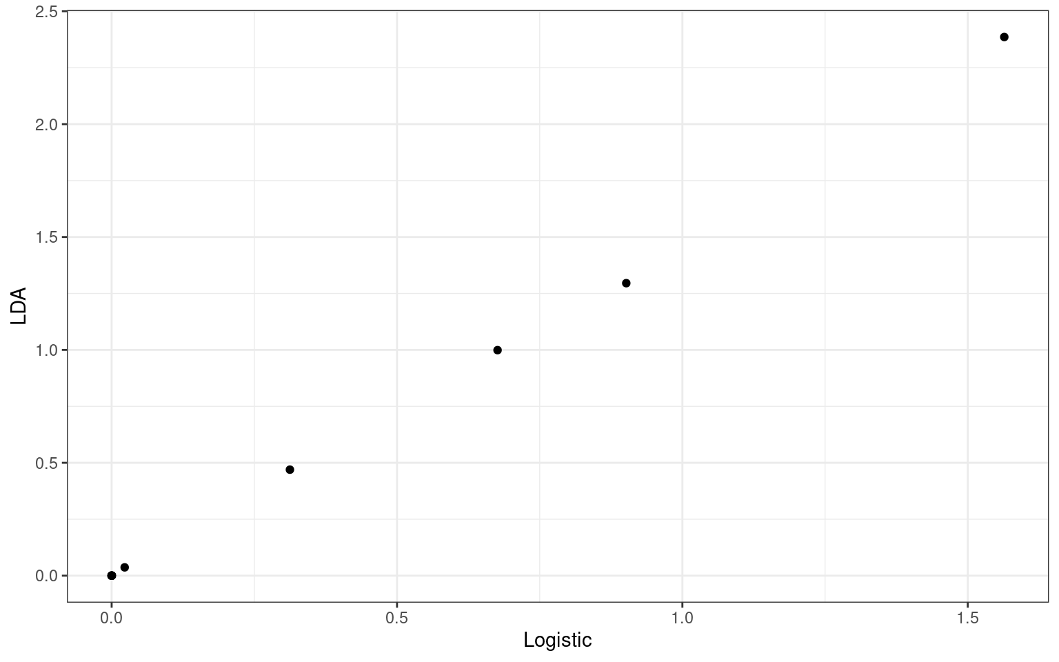
Here, the coefficients from the logistic and lda models are not identical, but their correlation is 1.0! If we compare the predicted probability vs. the lda likelihood, we see that they are highly correlated.
logit <- function(lo) {
1/(1 + exp(-lo))
} ##This is the inverse of the logodds function. The
df <- data.frame(logistic = predict(model1), lda = (predict(ll)$x)[, 1], logisticprob = logit(predict(model1)),
ldaprob = predict(ll)$posterior[, 2])
ggplot(df, aes(x = logistic, y = lda)) + geom_point() + theme_bw() + ggtitle("Logistic model vs LDA")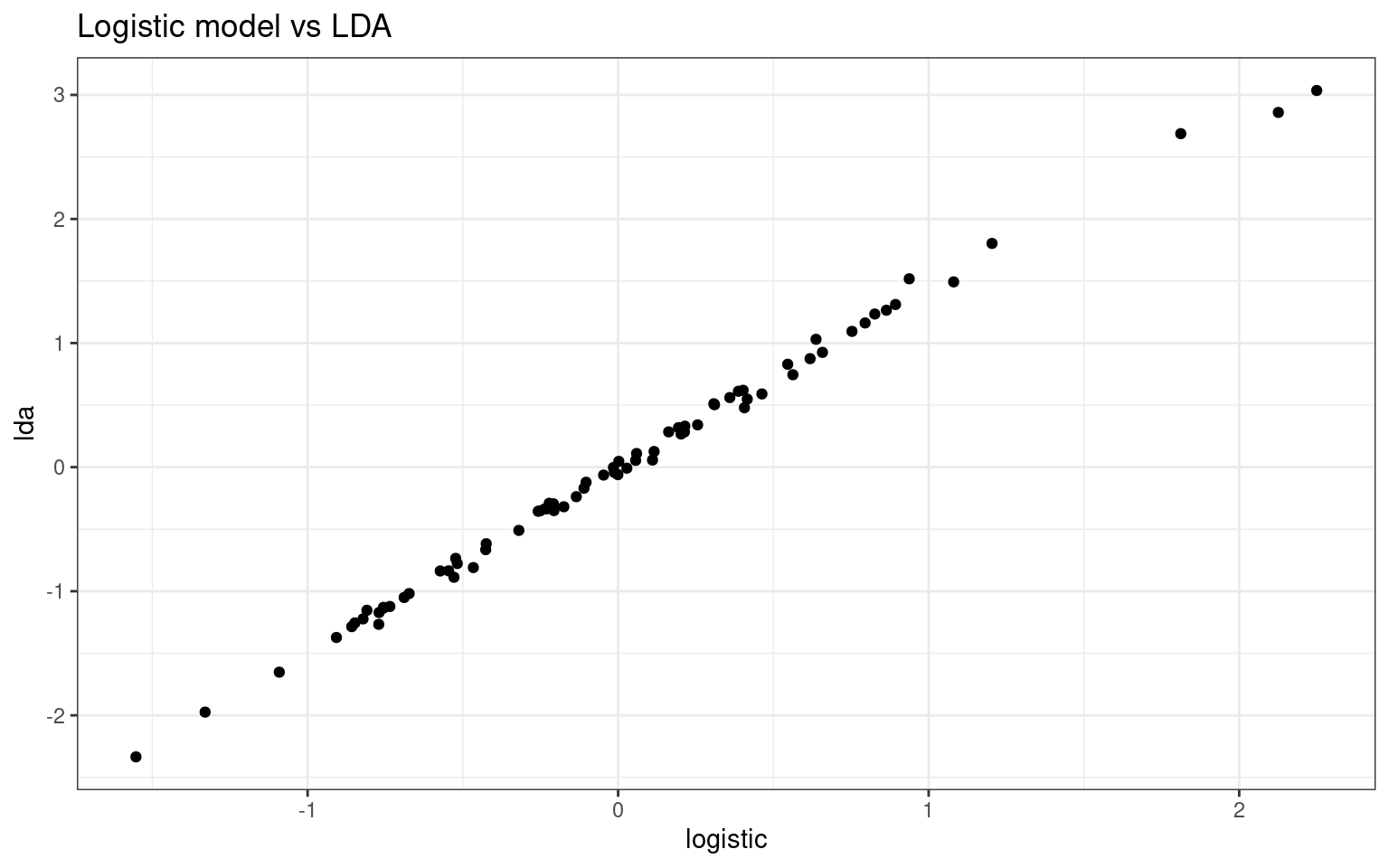
ggplot(df, aes(x = logisticprob, y = ldaprob)) + geom_point() + theme_bw() + ggtitle("Logistic probability vs LDA probability")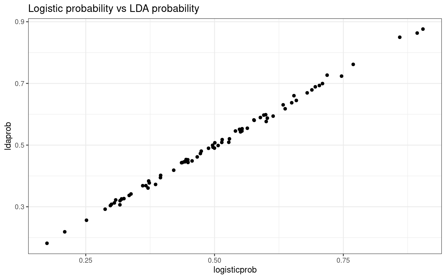
Notice how the discriminant value is almost the same as the log-odds predicted value in logistic regression, and transforming these to probabilities also produces almost identical values.
In terms of classification performance, the prediction for LDA was 1 error less than logistic regression, but the two models are really essentially identical, with the main difference being how the parameters are fit and the assumptions being made.
Cross-validation
It is easy to over-fit classification data, and so we must be careful to avoid this. Generally, just as with variable selection in regression models, we are worried about determining the best subset of predictors to use. Since using more variables will never make the model worse at fitting its own data, it is useful to hold some data out and test the model on the held-out data. A common approach is to use leave-one-out cross-validation. This approach will fit the model N times for N observations, fitting each left-out case in each model.
The LDA model allows you to do this automatically using the CV=TRUE
option. This will do the classification automatically, instead of
embedding it within the predict function and doing it
manually.
Results of original (overfit) model
Overall accuracy = 0.671

Confusion matrix
      Predicted (cv)
Actual  [,1]  [,2]
  [1,] 0.711 0.289
[2,] 0.368 0.632[1] 51Results of cross-validated model
Overall accuracy = 0.461

Confusion matrix
      Predicted (cv)
Actual     0     1
     0 0.465 0.535
1 0.545 0.455[1] 35Comparison of two models’ predictions
Overall accuracy = 0.789

Confusion matrix
      Predicted (cv)
Actual     0     1
     0 0.791 0.209
1 0.212 0.788[1] 60In contrast to the 51 cases we got correct before, the cross-validation gets just 35 correct (out of 76)–this is actually worse than chance! This is in spite of the fact that there is a lot of agreement between the two models. This poorer performance is telling us that the full model is overfitting the data.
Notice that we no longer have a single lda model to look at. The output of the cross-validation is simpler. We can’t look at the linear discriminant values or means because there is no longer one model–we tested N models.
$class
 [1] 0 0 0 1 1 0 0 0 1 0 0 0 1 0 1 0 1 1 1 0 0 1 0 0 0 1 0 0 0 1 0 0 1 0 0 1 1 0
[39] 1 0 0 1 0 1 0 0 0 1 0 1 0 0 1 1 0 1 1 1 1 1 0 1 0 1 0 0 1 1 0 1 1 0 0 1 0 0
Levels: 0 1

$posterior
            0         1
11  0.7932692 0.2067308
12  0.5469743 0.4530257
13  0.6111616 0.3888384
22  0.1626239 0.8373761
31  0.1460898 0.8539102
32  0.6590130 0.3409870
33  0.5343306 0.4656694
41  0.6910390 0.3089610
51  0.1772707 0.8227293
52  0.5495802 0.4504198
61  0.5799697 0.4200303
62  0.7598981 0.2401019
63  0.4867715 0.5132285
64  0.7752926 0.2247074
71  0.4180372 0.5819628
81  0.5583747 0.4416253
101 0.4326410 0.5673590
102 0.3218178 0.6781822
104 0.2705828 0.7294172
201 0.7983831 0.2016169
202 0.5647722 0.4352278
203 0.2553252 0.7446748
301 0.5082852 0.4917148
302 0.6851039 0.3148961
303 0.5797293 0.4202707
304 0.2312416 0.7687584
401 0.5506530 0.4493470
402 0.5486566 0.4513434
501 0.5358578 0.4641422
502 0.3694875 0.6305125
503 0.8212536 0.1787464
504 0.5295038 0.4704962
505 0.4794108 0.5205892
507 0.6428161 0.3571839
508 0.5490367 0.4509633
509 0.4697326 0.5302674
510 0.4345844 0.5654156
 [ reached getOption("max.print") -- omitted 39 rows ]

$terms
eng ~ eer + eeu + ep + ppr + ppu + eer.1 + eeu.1 + ep.1 + ppr.1 +
    ppu.1
attr(,"variables")
list(eng, eer, eeu, ep, ppr, ppu, eer.1, eeu.1, ep.1, ppr.1,
    ppu.1)
attr(,"factors")
      eer eeu ep ppr ppu eer.1 eeu.1 ep.1 ppr.1 ppu.1
eng     0   0  0   0   0     0     0    0     0     0
eer     1   0  0   0   0     0     0    0     0     0
eeu     0   1  0   0   0     0     0    0     0     0
ep      0   0  1   0   0     0     0    0     0     0
ppr     0   0  0   1   0     0     0    0     0     0
ppu     0   0  0   0   1     0     0    0     0     0
eer.1   0   0  0   0   0     1     0    0     0     0
 [ reached getOption("max.print") -- omitted 4 rows ]
attr(,"term.labels")
 [1] "eer"   "eeu"   "ep"    "ppr"   "ppu"   "eer.1" "eeu.1" "ep.1"  "ppr.1"
[10] "ppu.1"
attr(,"order")
 [1] 1 1 1 1 1 1 1 1 1 1
attr(,"intercept")
[1] 1
attr(,"response")
[1] 1
attr(,".Environment")
<environment: R_GlobalEnv>
attr(,"predvars")
list(eng, eer, eeu, ep, ppr, ppu, eer.1, eeu.1, ep.1, ppr.1,
    ppu.1)
attr(,"dataClasses")
      eng       eer       eeu        ep       ppr       ppu     eer.1     eeu.1
"numeric" "numeric" "numeric" "numeric" "numeric" "numeric" "numeric" "numeric"
     ep.1     ppr.1     ppu.1
"numeric" "numeric" "numeric"

$call
lda(formula = eng ~ ., data = joint, CV = TRUE)

$xlevels
named list()
The best practice in a situation like this might be to use cross-validation accuracy to help guide variable selection. You might use a stepwise procedure, and only include a variable if it improves cross-validation accuracy. You might use the single best model at the end, but still acknowledge cross-validation performance. In this case, results such as this led our research lab to conclude that there was no substantial difference between groups, and we developed new behavioral methods that were more powerful.
LDA with multiple categories
The other advantage of LDA over regression is that it handles
multiple categories directly. Here, just as with the
multinom() model, it creates \(N-1\) discriminant functions for \(N\) classes, each compared against a
baseline. Let’s look at the iris data for which we examined previously
under the multinomial model.
Call:
lda(Species ~ ., data = iris)

Prior probabilities of groups:
    setosa versicolor  virginica
 0.3333333  0.3333333  0.3333333

Group means:
           Sepal.Length Sepal.Width Petal.Length Petal.Width
setosa            5.006       3.428        1.462       0.246
versicolor        5.936       2.770        4.260       1.326
virginica         6.588       2.974        5.552       2.026

Coefficients of linear discriminants:
                    LD1         LD2
Sepal.Length  0.8293776 -0.02410215
Sepal.Width   1.5344731 -2.16452123
Petal.Length -2.2012117  0.93192121
Petal.Width  -2.8104603 -2.83918785

Proportion of trace:
   LD1    LD2
0.9912 0.0088
             setosa versicolor virginica
  setosa         50          0         0
  versicolor      0         48         2
  virginica       0          1        49
Now, the classification is very good, even with cross-validation. We can see two sets of coefficients–the two discriminant functions distinguishing each pairing of outcomes.
Quadratic Discriminant Analysis
One of the assumptions of LDA is that the two distributions have equal variance. If we relax this assumption, the best classification no longer has to be a line separating the space. We can get curved boundaries, or even a small region within a larger region. For example:
n <- 500
class <- rep(c("A", "B"), each = n)
x <- rnorm(n * 2, mean = rep(c(3, 4), each = n), sd = rep(c(0.25, 1), each = n))
y <- rnorm(n * 2, mean = rep(c(2.5, 1.5), each = n), sd = rep(c(0.25, 1), each = n))

qda1 <- qda(class ~ x + y, CV = TRUE)
table(class, qda1$class)
class   A   B
    A 490  10
B 35 465ggplot(data.frame(class, y, x), aes(x = x, y = y, colour = class)) + geom_point(size = 1.5) +
geom_density_2d() + geom_segment(x = -1, y = 6.5, xend = 7, yend = -1.5, col = "grey60",
lwd = 1.2) + geom_segment(x = 3, y = 2.5, xend = 4, yend = 1.5, col = "black",
lwd = 1.2) + coord_fixed(ratio = 1, xlim = c(0, 6), ylim = c(0, 6)) + ggtitle("Color by true class") +
theme_bw() + scale_color_manual(values = c("orange", "navy"))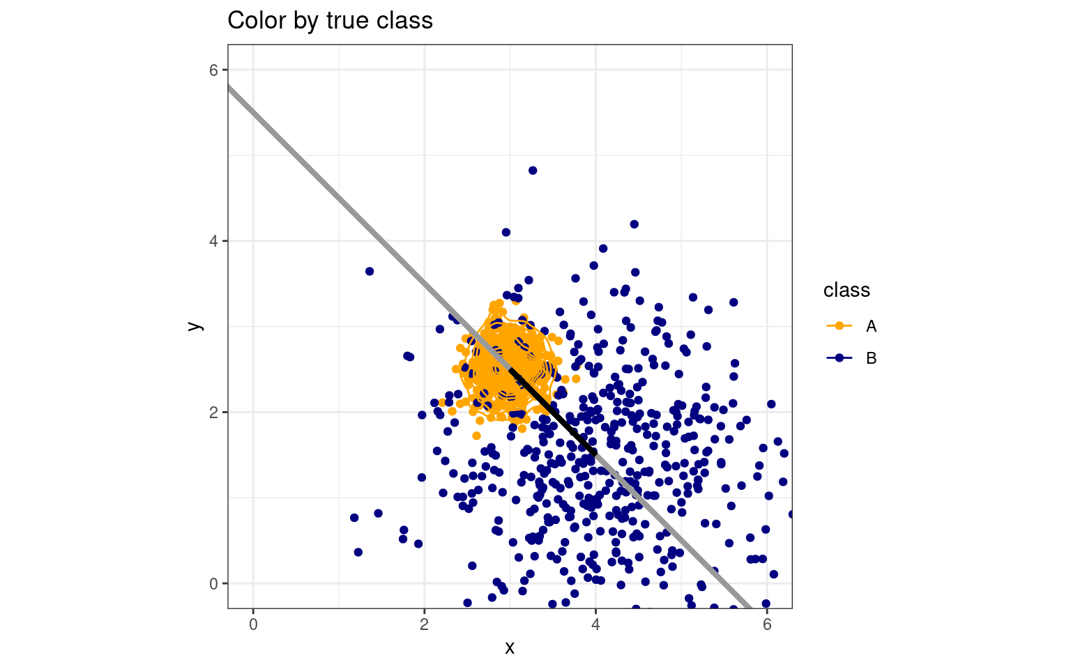
ggplot(data.frame(class, y, x), aes(x = x, y = y, colour = qda1$class)) + geom_point(size = 1.5) +
    geom_density_2d() + geom_segment(x = -1, y = 6.5, xend = 7, yend = -1.5, col = "grey60",
    lwd = 1.2) + geom_segment(x = 3, y = 2.5, xend = 4, yend = 1.5, col = "black",
    lwd = 1.2) + coord_fixed(ratio = 1, xlim = c(0, 6), ylim = c(0, 6)) + ggtitle("Colored by QDA classification") +
    theme_bw() + scale_color_manual(values = c("orange", "navy"))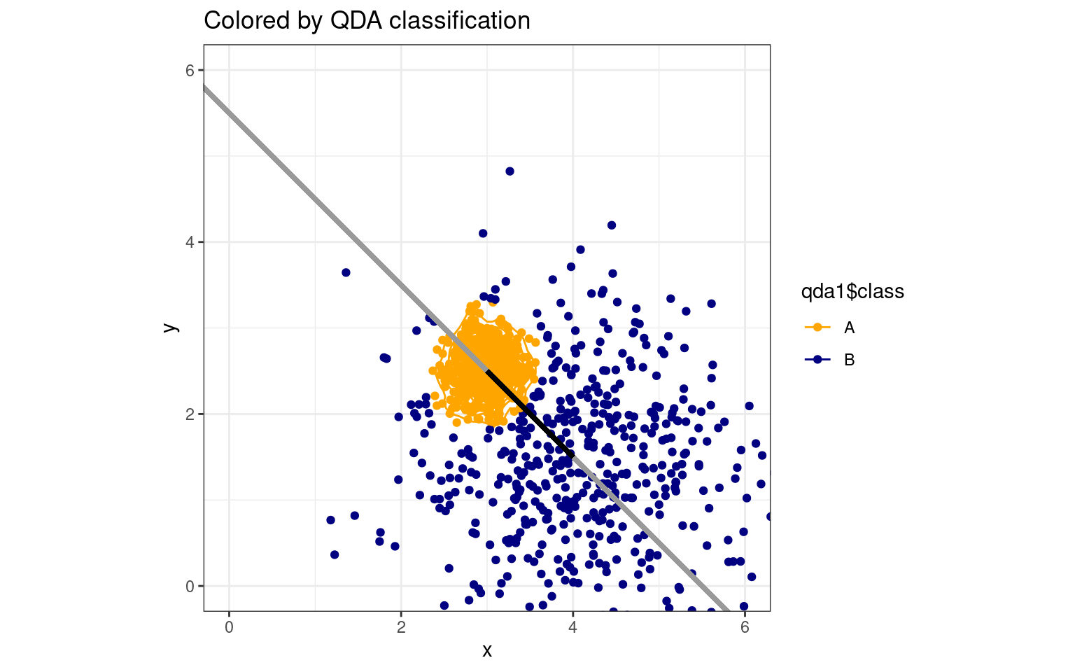
We can see how an LDA model will suffer. If all points are projected onto the discriminant line, the single boundary on that line will not be ideal. If we were able to make a curved boundary in this xy space, we could capture correct classifications. Quadratic Discriminant Analysis (QDA) permits this. It provides a more powerful classifier that can capture non-linear boundaries in the feature space. Thus, it is also less constrained, so requires more careful analysis to ensure we don’t overfit the model. How does it work with our real data set?
$class
 [1] 0 1 0 1 1 0 0 0 0 1 0 0 1 1 1 0 0 0 1 0 0 0 0 1 1 1 0 0 1 1 0 0 0 0 1 0 0 0
[39] 1 1 0 0 0 1 0 0 0 1 1 0 1 0 1 0 1 1 0 1 1 1 0 0 0 1 0 0 0 0 1 1 1 0 0 1 0 0
Levels: 0 1

$posterior
               0            1
11  9.974693e-01 2.530667e-03
12  8.815744e-02 9.118426e-01
13  9.472289e-01 5.277114e-02
22  1.370973e-01 8.629027e-01
31  1.379738e-16 1.000000e+00
32  9.478123e-01 5.218767e-02
33  7.036601e-01 2.963399e-01
41  7.048625e-01 2.951375e-01
51  1.000000e+00 1.103873e-08
52  3.288272e-01 6.711728e-01
61  8.394071e-01 1.605929e-01
62  9.297141e-01 7.028591e-02
63  4.762053e-01 5.237947e-01
64  5.772267e-02 9.422773e-01
71  1.996504e-03 9.980035e-01
81  7.733766e-01 2.266234e-01
101 8.181787e-01 1.818213e-01
102 7.929339e-01 2.070661e-01
104 1.165120e-03 9.988349e-01
201 9.983142e-01 1.685776e-03
202 6.645369e-01 3.354631e-01
203 6.743729e-01 3.256271e-01
301 9.814788e-01 1.852123e-02
302 1.627353e-05 9.999837e-01
303 2.929281e-01 7.070719e-01
304 3.462853e-02 9.653715e-01
401 6.924185e-01 3.075815e-01
402 9.115441e-01 8.845587e-02
501 4.643224e-01 5.356776e-01
502 4.199688e-01 5.800312e-01
503 9.999999e-01 1.320222e-07
504 8.343022e-01 1.656978e-01
505 8.036457e-01 1.963543e-01
507 8.672052e-01 1.327948e-01
508 7.843539e-05 9.999216e-01
509 6.728246e-01 3.271754e-01
510 8.772416e-01 1.227584e-01
 [ reached getOption("max.print") -- omitted 39 rows ]

$terms
eng ~ eer + eeu + ep + ppr + ppu + eer.1 + eeu.1 + ep.1 + ppr.1 +
    ppu.1
attr(,"variables")
list(eng, eer, eeu, ep, ppr, ppu, eer.1, eeu.1, ep.1, ppr.1,
    ppu.1)
attr(,"factors")
      eer eeu ep ppr ppu eer.1 eeu.1 ep.1 ppr.1 ppu.1
eng     0   0  0   0   0     0     0    0     0     0
eer     1   0  0   0   0     0     0    0     0     0
eeu     0   1  0   0   0     0     0    0     0     0
ep      0   0  1   0   0     0     0    0     0     0
ppr     0   0  0   1   0     0     0    0     0     0
ppu     0   0  0   0   1     0     0    0     0     0
eer.1   0   0  0   0   0     1     0    0     0     0
 [ reached getOption("max.print") -- omitted 4 rows ]
attr(,"term.labels")
 [1] "eer"   "eeu"   "ep"    "ppr"   "ppu"   "eer.1" "eeu.1" "ep.1"  "ppr.1"
[10] "ppu.1"
attr(,"order")
 [1] 1 1 1 1 1 1 1 1 1 1
attr(,"intercept")
[1] 1
attr(,"response")
[1] 1
attr(,".Environment")
<environment: R_GlobalEnv>
attr(,"predvars")
list(eng, eer, eeu, ep, ppr, ppu, eer.1, eeu.1, ep.1, ppr.1,
    ppu.1)
attr(,"dataClasses")
      eng       eer       eeu        ep       ppr       ppu     eer.1     eeu.1
"numeric" "numeric" "numeric" "numeric" "numeric" "numeric" "numeric" "numeric"
     ep.1     ppr.1     ppu.1
"numeric" "numeric" "numeric"

$call
qda(formula = eng ~ ., data = joint, CV = TRUE)

$xlevels
named list()Overall accuracy = 0.566
Confusion matrix
Predicted (cv)
Actual 0 1
0 0.556 0.444
1 0.419 0.581[1] 43Now, the qda model is a reasonable improvement over the LDA model–even with Cross-validation. We were at 46% accuracy with cross-validation, and now we are at 57%. This increased cross-validation accuracy from 35 to 43 accurate cases.
Variable Selection in LDA
We now have a good measure of how well this model is doing. But we suspect that–at least for LDA, the predictors might be over-fitting. We’d like to try removing variables to see if we get a better cross-validation performance. We could do this by hand, or using some tools built for this. The stepclass function within klaR package will do this:
correctness rate: 0.57857;  in: "ppr";  variables (1): ppr

 hr.elapsed min.elapsed sec.elapsed
0.000 0.000 0.235 method : lda
final model : eng ~ ppr
<environment: 0x564ee5418060>
correctness rate = 0.5786 correctness rate: 0.59286; in: "eeu.1"; variables (1): eeu.1
hr.elapsed min.elapsed sec.elapsed
0.000 0.000 0.231 method : qda
final model : eng ~ eeu.1
<environment: 0x564ee3500680>
correctness rate = 0.5929 If you run this several times, you will find that you get a slightly different model each time. The best models have 1 to 2 predictors, and vary in accuracy from 55 to 65%. This is happening because the cross-validation the method uses is somewhat random, so the best model will depend on how the cross-validation is initialized. Perhaps if we reduce the improvement required, and use a higher cross-validation value, we will end up at a more stable result. Using fold=76 should be similar to doing leave-one-out cross-validation, and using a smaller improvement criterion will avoid stopping early.
modelstepL <- stepclass(eng ~ ., "lda", direction = "both", data = joint, improvement = 0.001,
    fold = 76)
correctness rate: 0.57895; in: "ppr"; variables (1): ppr
correctness rate: 0.59211; in: "ppu"; variables (2): ppr, ppu
correctness rate: 0.60526; in: "ppu.1"; variables (3): ppr, ppu, ppu.1
hr.elapsed min.elapsed sec.elapsed
0.000 0.000 3.276 method : lda
final model : eng ~ ppr + ppu + ppu.1
<environment: 0x5b3643003ad0>
correctness rate = 0.6053 modelstepQ <- stepclass(eng ~ ., "qda", direction = "both", data = joint, improvement = 0.001,
fold = 76)correctness rate: 0.57895; in: "ppr"; variables (1): ppr
correctness rate: 0.64474; in: "ep"; variables (2): ppr, ep
hr.elapsed min.elapsed sec.elapsed
0.00 0.00 2.27 method : qda
final model : eng ~ ep + ppr
<environment: 0x5b36432bd030>
correctness rate = 0.6447 Now, the each model tends to converge on the same result each time. Recognize that the ‘best’ model is out there and does not change, but we just don’t always find it because the search involves randomness. However, oftentimes we get to a model that is basically as good as the best model. In small variable sets like this, we could examine every possible sub-model, but if you start moving to large models with thousands of variables, you will probably never find the exact best model. However, there is likely to be so much redundancy in those predictors that it does not really matter.
In our example, the variables selected are different for the two models, but that is probably fine. We can refit the best models using lda and qda to get more details about the fit:
Call:
lda(eng ~ ppr + ppu + ppu.1, data = joint)

Prior probabilities of groups:
  0   1
0.5 0.5

Group means:
        ppr       ppu    ppu.1
0 0.5789474 0.6052632 3007.688
1 0.6754386 0.7017544 3432.817

Coefficients of linear discriminants:
               LD1
ppr   1.2417704238
ppu   2.5194768800
ppu.1 0.0004672492Call:
qda(eng ~ ep + ppr, data = joint)
Prior probabilities of groups:
0 1
0.5 0.5
Group means:
ep ppr
0 0.6951754 0.5789474
1 0.6973684 0.6754386Example: LDA on the iphone data set
The following works through all the steps of LDA and QDA again with the iphone data set.
Data Preprocessing
Get rid of the gender variable, because it is categorical and LDA does not like that. It is also highly predictive, so this will help us see how good we can get.
Rescale all the numeric variables.
Compute LDA without Cross validation
Call:
lda(Smartphone ~ ., data = phone_type)

Prior probabilities of groups:
  Android    iPhone
0.4139887 0.5860113

Group means:
               Age Honesty.Humility Emotionality Extraversion Agreeableness
Android  0.2071126        0.2304728   -0.1885209  -0.08233383    0.04975669
iPhone  -0.1463150       -0.1628179    0.1331809   0.05816486   -0.03515069
        Conscientiousness    Openness Avoidance.Similarity
Android       -0.02859348  0.11922875            0.1678358
iPhone         0.02019991 -0.08422934           -0.1185679
        Phone.as.status.object Social.Economic.Status Time.owned.current.phone
Android             -0.2850676            -0.02423018               0.06110396
iPhone               0.2013865             0.01711745              -0.04316699

Coefficients of linear discriminants:
                                 LD1
Age                      -0.24833268
Honesty.Humility         -0.45905620
Emotionality              0.34275770
Extraversion              0.32566258
Agreeableness             0.01021013
Conscientiousness         0.26431245
Openness                 -0.15490974
Avoidance.Similarity     -0.29824541
Phone.as.status.object    0.38353264
Social.Economic.Status   -0.06839454
Time.owned.current.phone -0.01885251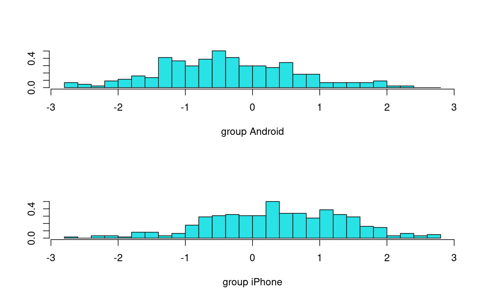
Predict using phone_type
Overall accuracy = 0.673

Confusion matrix
      Predicted (cv)
Actual  [,1]  [,2]
  [1,] 0.484 0.516
  [2,] 0.194 0.806
This looks reasonably good: 67% accuracy. Notably, it gets MOST android phones wrong, but by calling 80.6% of iphones correctly, it makes up for it. This is mostly because of the large overlap between the discriminant distributions.
Compute LDA with Cross-validation
One way to avoid over-fitting is to use leave-one-out cross-validation (LOOC). In this CV method, we repeatedly leave an observation out and fit the model with the remaining data, and testing and try to optimize parameters based on the accuracy of these missing values. This is bound to give poorer performance than the non-cross-validation version, but it will help us remove and select variables to make a better model when applied to new data. For LDA and QDA, CV=TRUE uses LOOC to fit its model.
$class
 [1] iPhone  iPhone  Android iPhone  Android iPhone  iPhone  Android iPhone
[10] iPhone  Android iPhone  iPhone  Android iPhone  iPhone  Android iPhone
[19] Android Android Android Android iPhone  iPhone  iPhone  Android Android
[28] iPhone  Android iPhone  iPhone  Android iPhone  iPhone  iPhone  Android
[37] iPhone  iPhone  iPhone  iPhone  iPhone  iPhone  iPhone  iPhone  iPhone
[46] iPhone  iPhone  iPhone  iPhone  Android iPhone  iPhone  iPhone  Android
[55] iPhone  iPhone  Android iPhone  Android iPhone  iPhone  Android Android
[64] iPhone  Android iPhone  iPhone  iPhone  Android iPhone  Android Android
[73] iPhone  iPhone  iPhone
 [ reached getOption("max.print") -- omitted 454 entries ]
Levels: Android iPhone

$posterior
       Android    iPhone
1   0.44727912 0.5527209
2   0.44682280 0.5531772
3   0.77836711 0.2216329
4   0.36991321 0.6300868
5   0.80731292 0.1926871
6   0.28517134 0.7148287
7   0.26967843 0.7303216
8   0.62504334 0.3749567
9   0.30966026 0.6903397
10  0.38754803 0.6124520
11  0.50156460 0.4984354
12  0.29046062 0.7095394
13  0.43235762 0.5676424
14  0.69385166 0.3061483
15  0.35384079 0.6461592
16  0.32701994 0.6729801
17  0.51765170 0.4823483
18  0.26246323 0.7375368
19  0.56630053 0.4336995
20  0.74414226 0.2558577
21  0.59475013 0.4052499
22  0.58309407 0.4169059
23  0.41664815 0.5833518
24  0.24077709 0.7592229
25  0.31182798 0.6881720
26  0.73235151 0.2676485
27  0.55432598 0.4456740
28  0.41271310 0.5872869
29  0.56705971 0.4329403
30  0.22477284 0.7752272
31  0.39035268 0.6096473
32  0.53711910 0.4628809
33  0.27895785 0.7210422
34  0.18762229 0.8123777
35  0.13193830 0.8680617
36  0.74365126 0.2563487
37  0.11854692 0.8814531
 [ reached getOption("max.print") -- omitted 492 rows ]

$terms
Smartphone ~ Age + Honesty.Humility + Emotionality + Extraversion +
    Agreeableness + Conscientiousness + Openness + Avoidance.Similarity +
    Phone.as.status.object + Social.Economic.Status + Time.owned.current.phone
attr(,"variables")
list(Smartphone, Age, Honesty.Humility, Emotionality, Extraversion,
    Agreeableness, Conscientiousness, Openness, Avoidance.Similarity,
    Phone.as.status.object, Social.Economic.Status, Time.owned.current.phone)
attr(,"factors")
                         Age Honesty.Humility Emotionality Extraversion
Smartphone                 0                0            0            0
Age                        1                0            0            0
Honesty.Humility           0                1            0            0
Emotionality               0                0            1            0
Extraversion               0                0            0            1
Agreeableness              0                0            0            0
                         Agreeableness Conscientiousness Openness
Smartphone                           0                 0        0
Age                                  0                 0        0
Honesty.Humility                     0                 0        0
Emotionality                         0                 0        0
Extraversion                         0                 0        0
Agreeableness                        1                 0        0
                         Avoidance.Similarity Phone.as.status.object
Smartphone                                  0                      0
Age                                         0                      0
Honesty.Humility                            0                      0
Emotionality                                0                      0
Extraversion                                0                      0
Agreeableness                               0                      0
                         Social.Economic.Status Time.owned.current.phone
Smartphone                                    0                        0
Age                                           0                        0
Honesty.Humility                              0                        0
Emotionality                                  0                        0
Extraversion                                  0                        0
Agreeableness                                 0                        0
 [ reached getOption("max.print") -- omitted 6 rows ]
attr(,"term.labels")
 [1] "Age"                      "Honesty.Humility"
 [3] "Emotionality"             "Extraversion"
 [5] "Agreeableness"            "Conscientiousness"
 [7] "Openness"                 "Avoidance.Similarity"
 [9] "Phone.as.status.object"   "Social.Economic.Status"
[11] "Time.owned.current.phone"
attr(,"order")
 [1] 1 1 1 1 1 1 1 1 1 1 1
attr(,"intercept")
[1] 1
attr(,"response")
[1] 1
attr(,".Environment")
<environment: R_GlobalEnv>
attr(,"predvars")
list(Smartphone, Age, Honesty.Humility, Emotionality, Extraversion,
    Agreeableness, Conscientiousness, Openness, Avoidance.Similarity,
    Phone.as.status.object, Social.Economic.Status, Time.owned.current.phone)
attr(,"dataClasses")
              Smartphone                      Age         Honesty.Humility
             "character"                "numeric"                "numeric"
            Emotionality             Extraversion            Agreeableness
               "numeric"                "numeric"                "numeric"
       Conscientiousness                 Openness     Avoidance.Similarity
               "numeric"                "numeric"                "numeric"
  Phone.as.status.object   Social.Economic.Status Time.owned.current.phone
               "numeric"                "numeric"                "numeric"

$call
lda(formula = Smartphone ~ ., data = phone_type, CV = TRUE)

$xlevels
named list()
confusion() on lda_mod2
We can examine the overall accuracy here via a confusion matrix as follows:
Overall accuracy = 0.648

Confusion matrix
      Predicted (cv)
Actual  [,1]  [,2]
  [1,] 0.466 0.534
  [2,] 0.223 0.777
We can see that some of the accuracy comes from overfitting. Without
CV, accuracy is 67%, and it goes down to 65%. This new model STILL gets
most android users wrong (and it gets worse in fact), and misses a few
more iPhone users. This seems like a bias in the decision, but let’s
think about how well the model could do if we didn’t use ANY predictors.
Suppose we just called all users iphone users in that case (note that
confusion breaks because it wants both categories in both
columns).
[1] 0.5860113So, we can get 59% correct by calling everyone an iPhone user, and 65% with LDA and CV, and 67% by overfitting LDA.
Compute QDA without CV
Just like LDA, applying qda alone does not use cross-validation. Consequently, it may overfit. Does it do better than LDA?
Call:
qda(Smartphone ~ ., data = phone_type)

Prior probabilities of groups:
  Android    iPhone
0.4139887 0.5860113

Group means:
               Age Honesty.Humility Emotionality Extraversion Agreeableness
Android  0.2071126        0.2304728   -0.1885209  -0.08233383    0.04975669
iPhone  -0.1463150       -0.1628179    0.1331809   0.05816486   -0.03515069
        Conscientiousness    Openness Avoidance.Similarity
Android       -0.02859348  0.11922875            0.1678358
iPhone         0.02019991 -0.08422934           -0.1185679
        Phone.as.status.object Social.Economic.Status Time.owned.current.phone
Android             -0.2850676            -0.02423018               0.06110396
iPhone 0.2013865 0.01711745 -0.04316699Overall accuracy = 0.682
Confusion matrix
Predicted (cv)
Actual [,1] [,2]
[1,] 0.53 0.47
[2,] 0.21 0.79Here, the QDA model is about 1% better than the LDA model without cross-validation. But let’s see if it is just better at fitting noise, or is it going to be better when we fit it with cross-validation.
Compute QDA with LOOC
Now, use CV=TRUE for the qda model:
$class
 [1] Android iPhone  Android iPhone  Android iPhone  iPhone  Android iPhone
[10] iPhone  iPhone  Android iPhone  Android iPhone  iPhone  iPhone  Android
[19] Android Android Android iPhone  iPhone  iPhone  iPhone  Android Android
[28] iPhone  Android iPhone  iPhone  iPhone  iPhone  iPhone  iPhone  Android
[37] iPhone  iPhone  iPhone  iPhone  iPhone  Android iPhone  iPhone  iPhone
[46] iPhone  iPhone  iPhone  iPhone  iPhone  iPhone  Android iPhone  Android
[55] iPhone  iPhone  Android Android Android iPhone  iPhone  iPhone  Android
[64] iPhone  iPhone  Android iPhone  iPhone  Android Android Android Android
[73] iPhone  Android iPhone
 [ reached getOption("max.print") -- omitted 454 entries ]
Levels: Android iPhone

$posterior
        Android       iPhone
1   0.550069334 4.499307e-01
2   0.459988979 5.400110e-01
3   0.758731421 2.412686e-01
4   0.373753872 6.262461e-01
5   0.509395253 4.906047e-01
6   0.223179114 7.768209e-01
7   0.046547074 9.534529e-01
8   0.629604274 3.703957e-01
9   0.155903266 8.440967e-01
10  0.404783055 5.952169e-01
11  0.390001107 6.099989e-01
12  0.527163938 4.728361e-01
13  0.277148516 7.228515e-01
14  0.668604563 3.313954e-01
15  0.352077947 6.479221e-01
16  0.241226583 7.587734e-01
17  0.442156078 5.578439e-01
18  0.712822007 2.871780e-01
19  0.629898021 3.701020e-01
20  0.653601501 3.463985e-01
21  0.537587845 4.624122e-01
22  0.365360338 6.346397e-01
23  0.486570165 5.134298e-01
24  0.053057264 9.469427e-01
25  0.223667837 7.763322e-01
26  0.791062415 2.089376e-01
27  0.682312320 3.176877e-01
28  0.338804289 6.611957e-01
29  0.541435101 4.585649e-01
30  0.159967108 8.400329e-01
31  0.283987762 7.160122e-01
32  0.251433765 7.485662e-01
33  0.188424179 8.115758e-01
34  0.203354196 7.966458e-01
35  0.149893921 8.501061e-01
36  0.504465263 4.955347e-01
37  0.057381722 9.426183e-01
 [ reached getOption("max.print") -- omitted 492 rows ]

$terms
Smartphone ~ Age + Honesty.Humility + Emotionality + Extraversion +
    Agreeableness + Conscientiousness + Openness + Avoidance.Similarity +
    Phone.as.status.object + Social.Economic.Status + Time.owned.current.phone
attr(,"variables")
list(Smartphone, Age, Honesty.Humility, Emotionality, Extraversion,
    Agreeableness, Conscientiousness, Openness, Avoidance.Similarity,
    Phone.as.status.object, Social.Economic.Status, Time.owned.current.phone)
attr(,"factors")
                         Age Honesty.Humility Emotionality Extraversion
Smartphone                 0                0            0            0
Age                        1                0            0            0
Honesty.Humility           0                1            0            0
Emotionality               0                0            1            0
Extraversion               0                0            0            1
Agreeableness              0                0            0            0
                         Agreeableness Conscientiousness Openness
Smartphone                           0                 0        0
Age                                  0                 0        0
Honesty.Humility                     0                 0        0
Emotionality                         0                 0        0
Extraversion                         0                 0        0
Agreeableness                        1                 0        0
                         Avoidance.Similarity Phone.as.status.object
Smartphone                                  0                      0
Age                                         0                      0
Honesty.Humility                            0                      0
Emotionality                                0                      0
Extraversion                                0                      0
Agreeableness                               0                      0
                         Social.Economic.Status Time.owned.current.phone
Smartphone                                    0                        0
Age                                           0                        0
Honesty.Humility                              0                        0
Emotionality                                  0                        0
Extraversion                                  0                        0
Agreeableness                                 0                        0
 [ reached getOption("max.print") -- omitted 6 rows ]
attr(,"term.labels")
 [1] "Age"                      "Honesty.Humility"
 [3] "Emotionality"             "Extraversion"
 [5] "Agreeableness"            "Conscientiousness"
 [7] "Openness"                 "Avoidance.Similarity"
 [9] "Phone.as.status.object"   "Social.Economic.Status"
[11] "Time.owned.current.phone"
attr(,"order")
 [1] 1 1 1 1 1 1 1 1 1 1 1
attr(,"intercept")
[1] 1
attr(,"response")
[1] 1
attr(,".Environment")
<environment: R_GlobalEnv>
attr(,"predvars")
list(Smartphone, Age, Honesty.Humility, Emotionality, Extraversion,
    Agreeableness, Conscientiousness, Openness, Avoidance.Similarity,
    Phone.as.status.object, Social.Economic.Status, Time.owned.current.phone)
attr(,"dataClasses")
              Smartphone                      Age         Honesty.Humility
             "character"                "numeric"                "numeric"
            Emotionality             Extraversion            Agreeableness
               "numeric"                "numeric"                "numeric"
       Conscientiousness                 Openness     Avoidance.Similarity
               "numeric"                "numeric"                "numeric"
  Phone.as.status.object   Social.Economic.Status Time.owned.current.phone
               "numeric"                "numeric"                "numeric"

$call
qda(formula = Smartphone ~ ., data = phone_type, CV = TRUE)

$xlevels
named list()
confusion() on qda_mod2
Overall accuracy = 0.594

Confusion matrix
      Predicted (cv)
Actual  [,1]  [,2]
  [1,] 0.420 0.580
  [2,] 0.284 0.716
Accuracy goes down to 59.4%, which compares to the 58.6% for the LDA. It looks like we get about a 1% boost in both cases.
Split-half and N-fold Cross Validation
LOOC can be computationally expensive if you have large data sets, and is not built into many classification schemes. A simpler scheme is to fit on one portion of the data and keep aside another portion for testing. We can do this repeatedly and get an overall estimate of accuracy. Sometimes, you might split your data into something like ten sets, and then fit the model ten times on 90% of the data and test on each 10% alone. This is called n-fold cross-validation; in this case 10-fold. Another scheme is to split the data in half, fitting on one half and testing on another. This would also be called split-half cross-validation. You can do this repeatedly on multiple different splits to get an average performance.
Below, I show a function will compute an lda and qda model, randomly picking half each time. The model fits on 1/2 of the data, and then predicts the other half. You could run this multiple times to get a better estimate of the fit of this class of model.
cv.lda <- function(class, predictors) {
    selection <- rep(c(T, F), length.out = length(class))[order(runif(length(class)))]
    out1 <- class[selection]
    pred1 <- predictors[selection, ]
    joint1 <- data.frame(out = out1, pred1)

    out2 <- class[!selection]
    pred2 <- predictors[!selection, ]
    joint2 <- data.frame(out = NA, pred2)

    ll <- lda(out ~ ., data = joint1)
    table(predict(ll, newdata = joint2)$class, out2)
    out.ll <- sum(diag(table(predict(ll, newdata = joint2)$class, out2)))/length(out2)
    qq <- qda(out ~ ., data = joint1)
    table(predict(qq, newdata = joint2)$class, out2)
    out.qq <- sum(diag(table(predict(qq, newdata = joint2)$class, out2)))/length(out2)

    c(out.ll, out.qq)
}

cv.lda(phone_type$Smartphone, phone_type[, 2:12])
[1] 0.6287879 0.5492424Each time we run this, we get a different pair of fits, so let’s try this 100 times and see how the two models compare.
out <- matrix(0, nrow = 250, ncol = 2)
for (i in 1:250) {
    cat(".")
    out[i, ] <- cv.lda(phone_type$Smartphone, phone_type[, 2:12])
}..........................................................................................................................................................................................................................................................[1] 0.6335303 0.5891212There is an advantage for the lda here, and it seems to perform a bit better that the previous models–around 63%! The story might be that qda’s extra parameters end up overfitting even with split-half CV, and that the simple model wins out.
Step from klaR
These models fit on the entire data set, but a good way to prevent
overfitting is to do variable selection. In classification, this is
referred to as feature selection and dimensionality reduction (although
that can sometimes use PCA). We can automate variable selection with
stepclass in the klaR library, which uses CV
to determine whether a variable should be kept. We can specify the
‘foldness’ of the CV: here we use 2-fold, but 4-fold would hold out 1/4
of the data and fit on the other 3/4.
library(klaR)
model <- stepclass(Smartphone ~ ., data = phone_type, method = "lda", fold = 2, start.vars = 1:11,
    direction = "both", output = T)
correctness rate: 0.6351; starting variables (11): Age, Honesty.Humility, Emotionality, Extraversion, Agreeableness, Conscientiousness, Openness, Avoidance.Similarity, Phone.as.status.object, Social.Economic.Status, Time.owned.current.phone
correctness rate: 0.64267; out: "Age"; variables (10): Honesty.Humility, Emotionality, Extraversion, Agreeableness, Conscientiousness, Openness, Avoidance.Similarity, Phone.as.status.object, Social.Economic.Status, Time.owned.current.phone
correctness rate: 0.65968; out: "Social.Economic.Status"; variables (9): Honesty.Humility, Emotionality, Extraversion, Agreeableness, Conscientiousness, Openness, Avoidance.Similarity, Phone.as.status.object, Time.owned.current.phone
correctness rate: 0.66349; out: "Agreeableness"; variables (8): Honesty.Humility, Emotionality, Extraversion, Conscientiousness, Openness, Avoidance.Similarity, Phone.as.status.object, Time.owned.current.phone
hr.elapsed min.elapsed sec.elapsed
0.000 0.000 0.427 modell2 <- lda(model$formula, data = phone_type)
confusion(phone_type$Smartphone, predict(modell2)$class)Overall accuracy = 0.679
Confusion matrix
Predicted (cv)
Actual [,1] [,2]
[1,] 0.498 0.502
[2,] 0.194 0.806Here, using variable selection and CV, our fit goes to 66.6% for the LDA model–the best fit yet. What about QDA?
modelq <- stepclass(Smartphone ~ ., data = phone_type, method = "qda", fold = 2,
    start.vars = 1:11, direction = "both", output = T)
correctness rate: 0.58598; starting variables (11): Age, Honesty.Humility, Emotionality, Extraversion, Agreeableness, Conscientiousness, Openness, Avoidance.Similarity, Phone.as.status.object, Social.Economic.Status, Time.owned.current.phone
correctness rate: 0.60113; out: "Honesty.Humility"; variables (10): Age, Emotionality, Extraversion, Agreeableness, Conscientiousness, Openness, Avoidance.Similarity, Phone.as.status.object, Social.Economic.Status, Time.owned.current.phone
correctness rate: 0.60675; out: "Extraversion"; variables (9): Age, Emotionality, Agreeableness, Conscientiousness, Openness, Avoidance.Similarity, Phone.as.status.object, Social.Economic.Status, Time.owned.current.phone
correctness rate: 0.62564; out: "Avoidance.Similarity"; variables (8): Age, Emotionality, Agreeableness, Conscientiousness, Openness, Phone.as.status.object, Social.Economic.Status, Time.owned.current.phone
hr.elapsed min.elapsed sec.elapsed
0.000 0.000 0.434 modelq2 <- qda(modelq$formula, data = phone_type)
confusion(phone_type$Smartphone, predict(modelq2)$class)Overall accuracy = 0.66
Confusion matrix
Predicted (cv)
Actual [,1] [,2]
[1,] 0.470 0.530
[2,] 0.206 0.794This appears to improve things even more–to 68.5%; by fitting a smaller model we actually do better. Originally, we had 11 predictor variables. Each time this is run, the result is a bit different, but in my case the lda dropped to 8, whereas the qda dropped to 9. They tended to remove different variables–lda removed agreeableness but kept the other personality variables and removed the variables avoidance of similarity, phone as status object, and socio-economic status, but QDA kept these and removed more personality variables. This might just be luck and not related to the greater complexity of qda. Multicolinearity could mean that there are mutually-exclusive sets of variables that provide roughly equivalent solutions, and if you start down one path early you end up with one set, but if you start down the other path you end up with the other set.
Smartphone ~ Honesty.Humility + Emotionality + Extraversion +
    Conscientiousness + Openness + Avoidance.Similarity + Phone.as.status.object +
    Time.owned.current.phone
<environment: 0x564ee02a56f0>Smartphone ~ Age + Emotionality + Agreeableness + Conscientiousness +
Openness + Phone.as.status.object + Social.Economic.Status +
Time.owned.current.phone
<environment: 0x564ee23200b8>Applications of LDA
Although the performance of LDA can often be surpassed by more modern machine learning methods, there are several reasons it still sees widespread use.
It is simple to use and understand. Like logistic regression, it can be used to make a simple model or decision tool that is both easy to implement and transparent.
It is sufficient for many situations. Many times, the benefit you might get from using a more complex model is negligible, at the cost of complexity or (worse yet) the possibility of making large mistakes because of strange interactions that you might not be able to predict.
Some of the most widely-used LDA models are within finance. For example, Altman’s (1968) bankruptcy model is based on LDA, predicting bankruptcy of firms within the next two years based on a handful of publicly-available statistics (see Altman, 1968, “Financial ratios, discriminant analysis and the prediction of corporate bankruptcy”. The Journal of Finance, 23(4), 589-609.) This is useful because the model can be implemented in a spreadsheet and the model’s parameters might be easily communicated so individuals can assess whether they want to invest in something.
Alternatives and extensions in Machine Classification
There are hundreds of special-purpose methods available for machine classification, many of which are developed for special kinds of situations or that work under different assumptions. We will cover several of these in this class, and here is a partial listing of methods you might want to be familiar with:
Within the klaR library, there are several implementations of related methods.
- rda: Regularized discriminant Analysis. Attempts to build a discriminant model that is more robust to correlation between predictors (multi-colinearity)
- Probabilistic LDA. This frames the LDA problem in a Bayesian and/or maximum likelihood format, and is increasingly used as part of deep neural nets as a ‘fair’ final decision that does not hide complexity.
- sknn: simple k-nearest-neighbors classification. Makes classification based on a vote of the nearest observations
- loclda: Makes a local lda for each point, based on its nearby neighbors. Similar to adding LDA to a KNN classifier, which we will discuss in an upcoming module.
- NaiveBayes: A common and simple classifier based on bayes rule
- svmlight: a lightweight ‘support vector machine’, which generalizes lda, focusing especially on identifying a good decision rule that separates the two groups
The klaR library also has a lot of functions to help with variable selection and cross-validation.
Within the nnet library:
- nnet: a neural net classifier–essentially a network of LDA classifiers or logistic regressions.
- multinom: an extension of generalized linear regression for multiple groups
Within the class library
- knn: a straightforward set of knn tools.