K-Nearest-Neighbor classifiers
K Nearest-Neighbor classifiers
K Nearest-Neighbor classifiers is a simple and special case of a case-based reasoning (CBR) system. In a CBR, you collect a case-base of examples, determine a way of measuring similarity between a new case and all cases in the case-base, and use the most similar cases to make a decision. CBR systems are used in many applications, including self-driving cars, medical diagnoses, and recommender systems. KNN is a simple CBR system that is used in many applications as well.
Nearest-neighbor methods are a class of non-model-based classifiers. It requires you to develop a way of measuring similarity or distance between the case you care about and all examples in your case-base–usually on the basis of a set of predictors or features. Once this distance space is defined, we determine the class by finding the closest few neighbors in that space, and having those neighbors vote, using the most common label of items in the neighborhood. Because this could be susceptible to noisy data, we usually find a set of \(k\) neighbors and have them vote on the outcome. These are K-nearest neighbor classifiers, or KNN. This approach can be especially useful if your data classes are not well described by a multivariate distribution. Ultimately, this means KNN approaches make fewer assumptions, but also have to make ad hoc assumptions about combining dimensions that may not be valid.
The problem with KNN is similar to many classifiers–how do we know which features to use. Furthermore, because we need to combine features to create a distance, we also need to come up with formulas for combining multiple features to create a distance measure. And this needs to be done for every pair of items before we start, so removing a variable means recomputing the entire similarity space. We may need to decide which features to use. Whether all dimensions should be equally weighted, how to normalize features that are on different scales. What if some of our features are categorical? Unlike something like logistic regression, we cannot easily test particular predictors, but we can always do cross-validation tests to determine whether the a decision in selecting variables or creating a distance metric improve outcomes.
Choosing K.
The choice of \(k\) can have a big impact on the results. If \(k\) is too small, classification will be highly impacted by local neighborhood; if it is too big (i.e., if \(K\) = \(N\)), it will always just respond with the most likely response in the entire population. We can do leave-one-out cross validation on our case-base to determine the best \(k\) value, and although this won’t necessarily be the best value to use for new cases, it should help us decide.
Calculating distance
The distance metric must be chosen so that we can compute the distance between our new case and every example in our case-base. There are a number of options, and the choice sometimes makes a difference, and some ways to do it will lead to problems. For example, if you want to decide on political party based on age, income level, and gender, you need to figure out how to weigh and combine these. By default, you might add differences along each dimension, which would combine something that differs on the scale of dozens with something that differs on the scale of thousands, and so the KNN model would essentially ignore gender and age. That is, if we used a city-block distance (summing each absolute difference), a 22-year-old female democrat who makes $30,000/year might be 2 units away from a 22-year-old male republican who also makes $30K, but 1,000 units away from a 22-year-old female republican who makes $31,000. But had we chosen to represent age in days and salary in thousands of dollars, we would get a completely different space. You might want to adjust the scale of different dimensions, select/ignore different dimensions, or weigh some more than others.
If we create a sample data set with randomly-generated people, coding
gender and party as 1 or 2 to allow us easier calculation of distance
using the dist function:
set.seed(100)
library(ggplot2)
vals <- data.frame(salary = sample(c(30000, 50000, 1e+05), 50, replace = T), gender = sample(1:2,
    50, replace = T), party = sample(1:2, 50, replace = T))
tmpdat <- data.frame(values = as.numeric(dist(vals)))

tmpdat |>
    ggplot(aes(x = values)) + geom_histogram() + theme_bw()
values
               0                1  1.4142135623731            20000
              89              206              107               61
    20000.000025      20000.00005            50000      50000.00001
             112               61               85              172
     50000.00002            70000 70000.0000071429 70000.0000142857
              85               62              126               59
Notice that there appear to be only 4 distances between cases, but looking more carefully we have a some other cases, e.g., 20000, 20000.00005, 20000.000025, etc. We might choose to normalize these somehow.
Normalization selection
A typical approach would be to normalize all variables first. Then
each variable has equal weight and range. We can normalize against the
entire range, or via z-scores. If you have multiple variables that are
on the same overall scale (i.e., a likert scale), you might apply the
same normalization to all variables. The scale function in
R can do this for a matrix of values:
vals2 <- scale(vals)
tmpdat <- data.frame(values = as.numeric(dist(vals2)))
tmpdat |>
    ggplot(aes(x = values)) + geom_histogram() + theme_bw()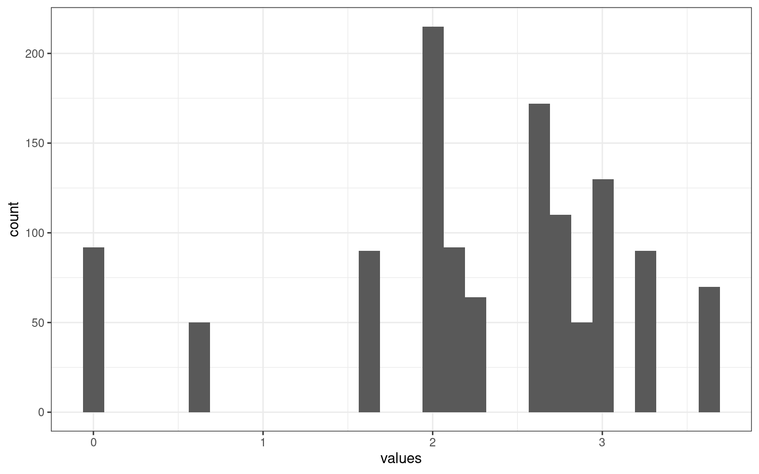
There is a much broader range here. But because gender and party have a max difference of 1, maybe we want salary to also be scaled similarly.
vals2 <- vals
vals2$salary <- (vals2$salary - min(vals2$salary))/(max(vals2$salary) - min(vals2$salary))
tmpdat <- data.frame(values = as.numeric(dist(vals2)))
tmpdat |>
ggplot(aes(x = values)) + geom_histogram() + theme_bw()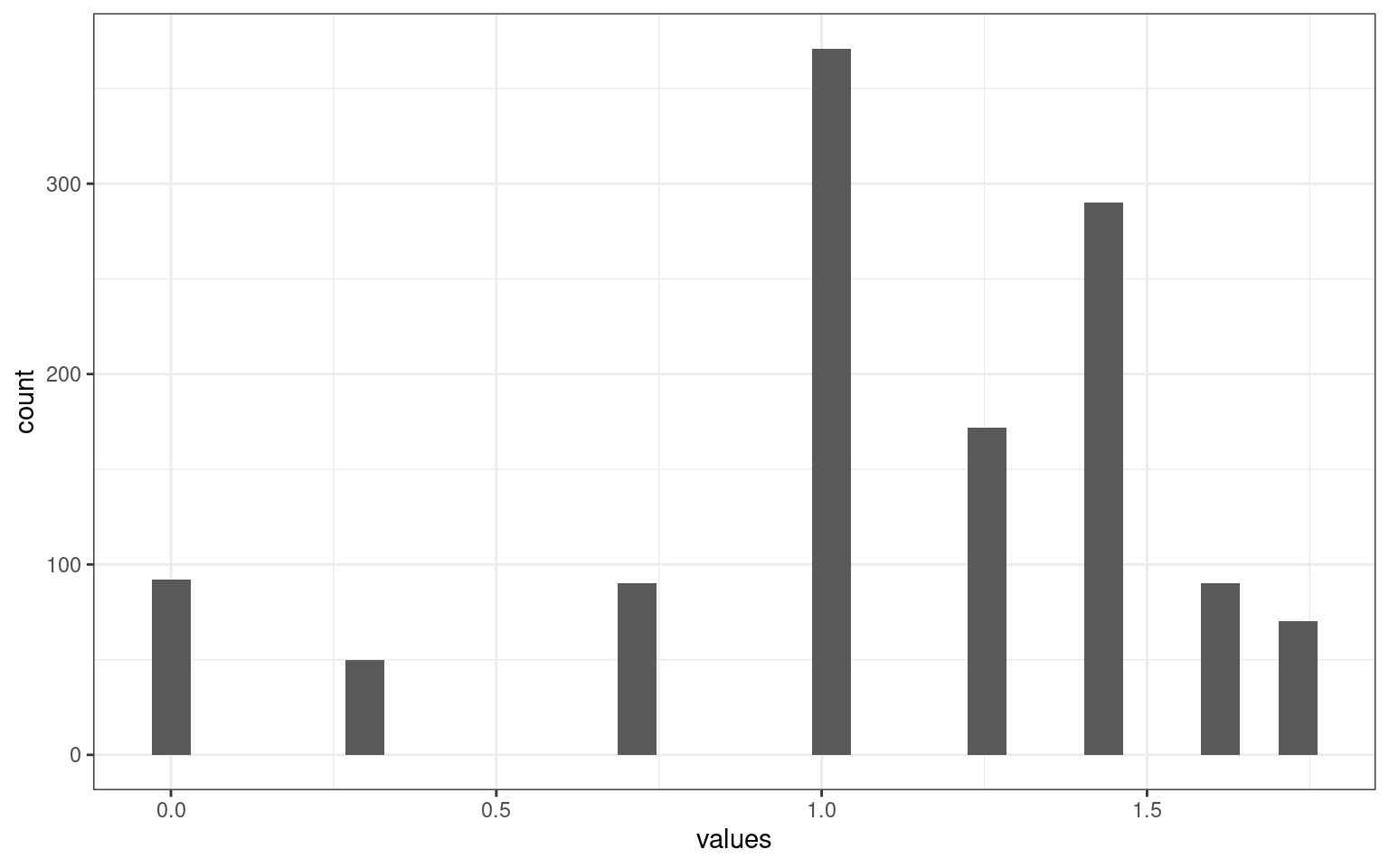 This measure is sort of like downweighting the role of salary. We could
similarly weigh dimensions unequally if we want, by multiplying the
feature values by a vector.
This measure is sort of like downweighting the role of salary. We could
similarly weigh dimensions unequally if we want, by multiplying the
feature values by a vector.
vals3 <- t((t(vals2) * c(0.33, 0.333, 0.33)))
tmpdat <- data.frame(values = as.numeric(dist(vals3)))
tmpdat |>
    ggplot(aes(x = values)) + geom_histogram() + theme_bw()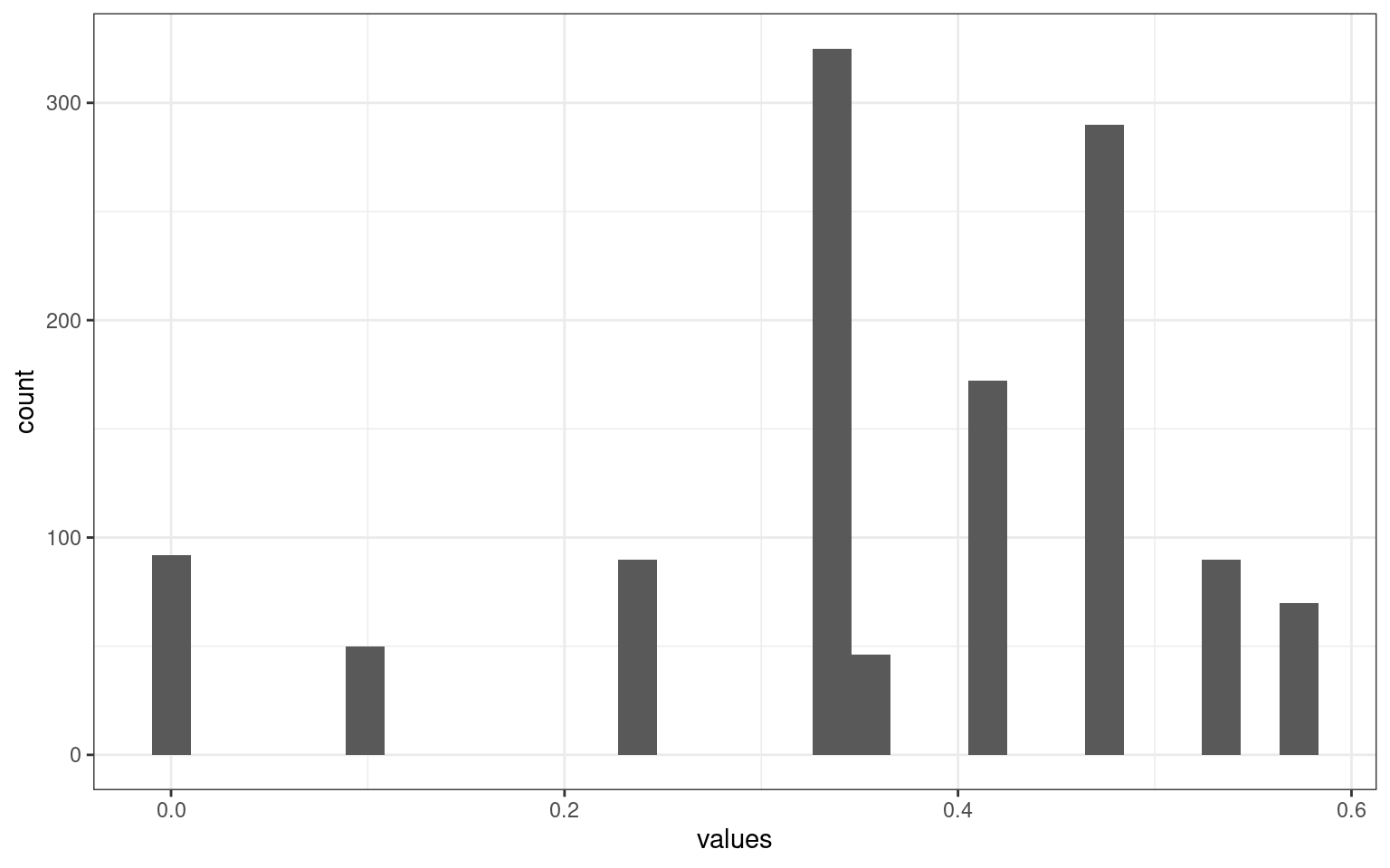
Alternative distance metrics
The dist() function provides a number of alternative
distance metrics. The most common metric is euclidean, calculating the
shortest distance as if the features were a space where you can move
diagonally. Another common metric is the manhattan or city-block metric,
which adds up distances on each feature. There are others, including
minkowski which provides a parameterized function that can scale from
min to median to max. A min or max distance might be reasonable because
they match the closest dimension or worst-case difference.
tmpdat <- data.frame(values = as.numeric(dist(vals2, method = "manhattan")))
tmpdat |>
    ggplot(aes(x = values)) + geom_histogram() + theme_bw() + ggtitle("Manhattan distance")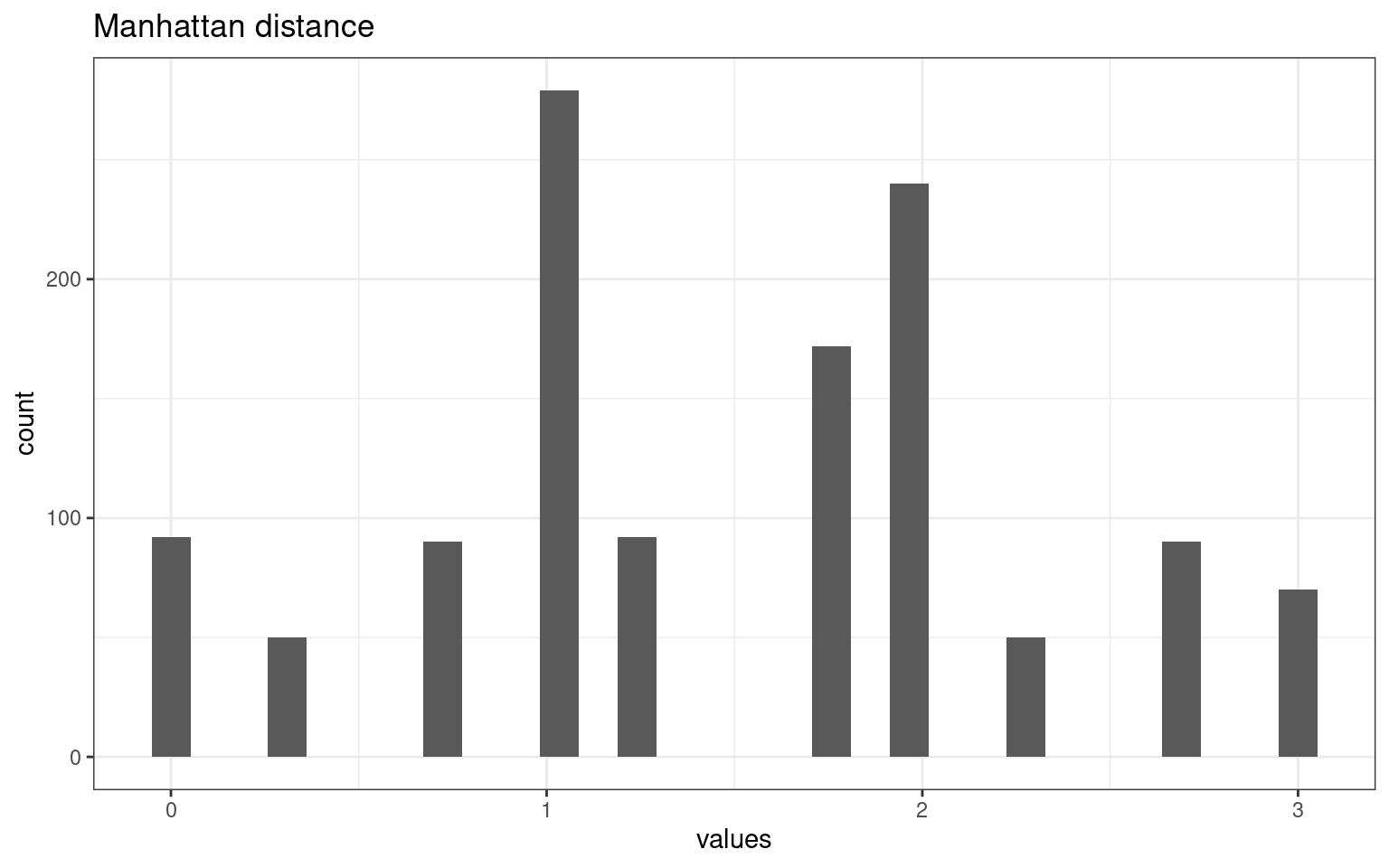
tmpdat <- data.frame(values = as.numeric(dist(vals2, method = "minkowski", p = 100)))
tmpdat |>
    ggplot(aes(x = values)) + geom_histogram() + theme_bw() + ggtitle("Minkowski distance p= 100 (max)")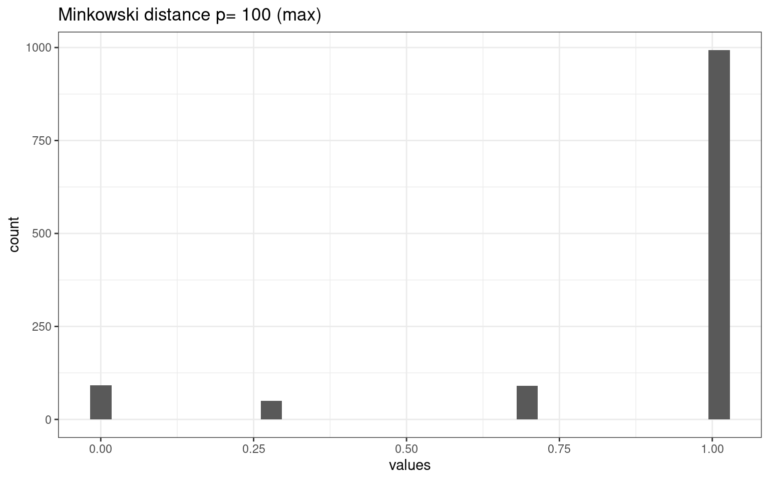
tmpdat <- data.frame(values = as.numeric(dist(vals2, method = "minkowski", p = 1/100)))
tmpdat |>
    ggplot(aes(x = values)) + geom_histogram() + theme_bw() + ggtitle("Minkowski distance p= 1/100 (min)")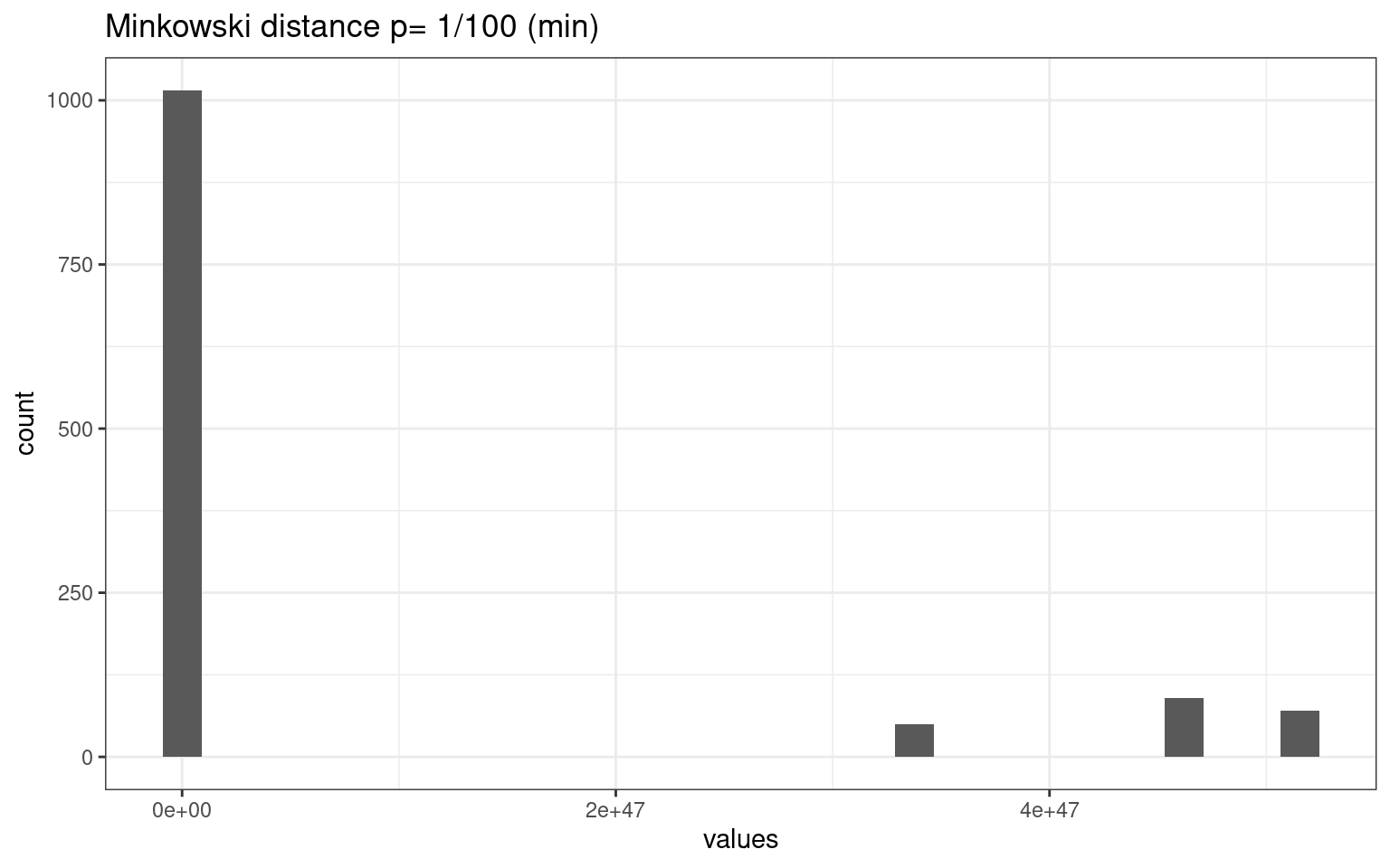
The different metrics produce very different distributions of distances among our cases. This make a big difference.
Using the knn function
Unlike previous methods where we train a system based on data and then make classifications, for KNN the trained system is just a set of cases–no statistics are actually calculated from it. A number of libraries and functions are available:
Libraries and functions.
There are several options for knn classifers.
Library: class
- Function: knn
- Function: knn.cv (cross-validation)
Library: kknn
- Function: kknn
- This provides a ‘weighted k-nearest neighbor classifier’. Here, weighting is a weighting kernel, which gives greater weights to the nearer neighbors.
Library: klaR
- Function: sknn
- A ‘simple’ knn function. Permits using a parameterized weighting kernel as well.
Cross-validation
Some of the libraries include cross-validation schemes, which is important. Because KNN is a non-parametric method, it is easy to overfit the data. Remember that we first calculate the distance between all points, which includes all dimensions. CV should be useful in helping us remove dimensions that are not useful, so if we do that, we have to re-compute the entire distance matrix which may not be easy.
The knn.cv function in the class library will do a
leave-one-out cross-validation. It reasonably does not consider the case
itself in making a decision (which would bias things), and if we just
tried to predict the data set from itself, the closest case would always
be itself, so it would always be correct if K=1, or higher than it
should be if K is larger.
Example
For our 50-case data set, suppose we want to use knn to predict gender based on party and salary. These are random, so we should not be able to do very well. Let’s try a simple knn(), which calculates the distance unweighted via euclidean distance:
library(DAAG)
library(class)
k1 <- knn(vals2[, -3], vals2[, -3], cl = vals2$party, k = 3)
confusion(k1, vals2$party)
Overall accuracy = 0.62
Confusion matrix
Predicted (cv)
Actual 1 2
1 0.64 0.36
2 0.40 0.60Here, we got 60% accuracy. This seems surprising because the data were random, but because we are predicting based on the same data we are using, and use a small \(k=3\), we are biasing the response by including the tested data in the training set. Here, using \(k=1\) doesn’t get perfect prediction because there are a lot of ties in the data in terms of gender and salary.
Overall accuracy = 0.56

Confusion matrix
      Predicted (cv)
Actual     1     2
     1 0.583 0.417
     2 0.462 0.538
Because our data set is clumpy (only 3 salaries), it could be worse–we could easily get 100% accuracy. We need to cross-validate.
We can use knn.cv to do a leave-one-out cross-validation
on \(knn\). That is, it fits each case
with all the other points and returns the results, avoiding using the
case itself as part of the voting.
Overall accuracy = 0.46

Confusion matrix
      Predicted (cv)
Actual     1     2
     1 0.478 0.522
     2 0.556 0.444
This provides results around 50% accurate, which is what we’d expect with random data. Note that knn.cv will not help you fit new data, but does give sort of an upper bound for how good the classifier might be, and may help evaluate which features to remove or include.
We might also do some cross-validation by hand, by holding 10 out and fitting them with the other 40:
test <- sample(1:50, 10)

testset <- vals2[test, ]
trainset <- vals2[-test, ]
k2 <- knn(trainset[, -3], testset[, -3], cl = trainset$party, k = 3)
confusion(k2, testset$party)
Overall accuracy = 0.9
Confusion matrix
Predicted (cv)
Actual 1 2
1 1.0 0.0
2 0.2 0.8Running this multiple times you will find that the average accuracy tends to be 50%, which is what we would expect.
iPhone data set example:
In general, we need to normalize the variables first when using
knn, because for the simplest knn we have no
control over the distance metrics.
phone <- read.csv("data_study1.csv")
# Normalizing the values by creating a new function
normal = function(x) {
    xn = (x - min(x))/(max(x) - min(x))
    return(xn)
}

phone$Gender <- as.numeric(as.factor(phone$Gender))


phone2 <- phone
for (i in 2:ncol(phone2)) {
    phone2[, i] = normal(as.numeric(phone2[, i]))
}

# we might also use scale:
phone3 <- scale(phone[, -(1)])

# checking the range of values after normalization
par(mfrow = c(1, 3), mar = c(2, 12, 1, 1))
boxplot(phone[, 2:12], main = "Original", horizontal = T, las = 1)
boxplot(phone2[, 2:12], main = "Using `normal`", horizontal = T, las = 1)
boxplot(phone3, main = "Using `scale`", horizontal = T, las = 1)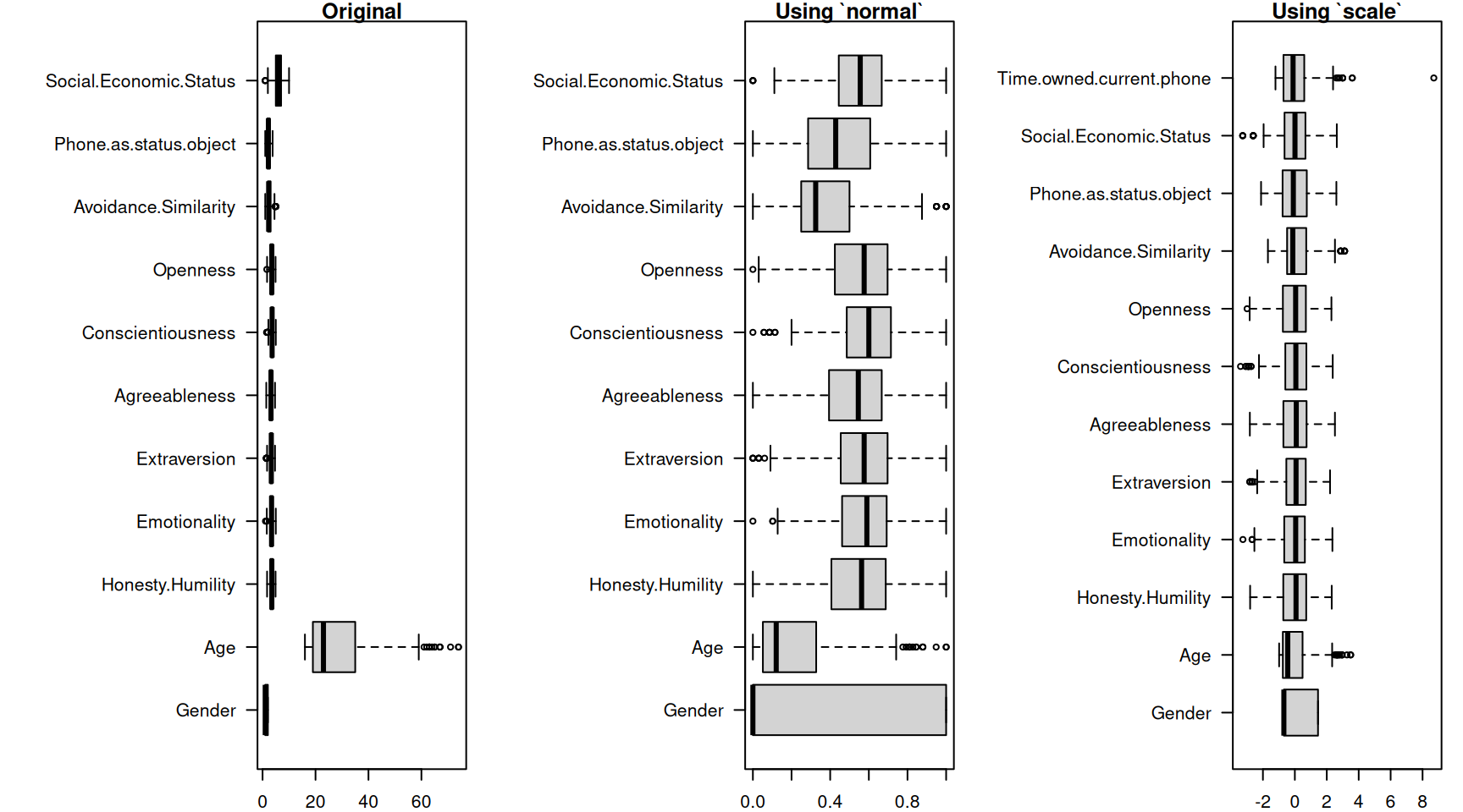
Fitting a simple KNN model
Here, we use the class:knn model. We specify separate
the training and testing separately, but they can be the same, and if we
use knn.cv it will exclude the point when making a classification.
Again, ‘training’ a knn is a bit deceptive, the training pool is just
the set of points being used to classify the test cases. We will use a k
of 11, which means each case will be compared to the 11 closes cases and
a decision made based on the vote of those. Using an odd number means
that there won’t be a tie.
library(class)
m1 = knn.cv(train = phone2[, -1], cl = phone2$Smartphone, k = 11)
confusion(phone2$Smartphone, m1)
Overall accuracy = 0.645
Confusion matrix
Predicted (cv)
Actual [,1] [,2]
[1,] 0.511 0.489
[2,] 0.261 0.739That is pretty good, but what if we expand k
Overall accuracy = 0.641

Confusion matrix
      Predicted (cv)
Actual  [,1]  [,2]
  [1,] 0.507 0.493
  [2,] 0.265 0.735
It looks we the choice of \(k\) is not going to matter much. What we could do is play with cross-validation though–right now we are testing on the same set as we are ‘training’ with, which will boost our accuracy (since the correct answer will always be one of the elements.) We can also try to do variable selection to change the similarity space to something that works better.
phone2 <- phone2[order(runif(nrow(phone2))), ]  #random sort
phone.train = phone2[1:450, 2:12]
phone.test = phone2[451:nrow(phone2), 2:12]
phone.train.target = phone2[1:450, 1]
phone.test.target = phone2[451:nrow(phone2), 1]

train <- sample(1:nrow(phone2), 300)
m2 <- knn(train = phone.train, test = phone.test, cl = phone.train.target, k = 10)
confusion(phone.test.target, m2)
Overall accuracy = 0.633
Confusion matrix
Predicted (cv)
Actual [,1] [,2]
[1,] 0.594 0.406
[2,] 0.340 0.660Split-half cross-validation and using alternate distances and kernels
The kknn:kknn function provides two advances: it uses a minkowski distance enabling you to set parameter p=2 (euclidian distance); p=1 (manhattan distance), or very large (max) or very close to 0 (min). In addition, the voting is done according to a specified ‘kernel’, so that you can weigh closer cases more strongly than farther cases. The standard knn uses a rectangular kernel, but kknn uses an ‘optimal’ kernel by default.
When we use this, we have to organize the test/train data a little differently, so I’ll split them into two data frames first.
kknn uses a regression-like formula to specify the trained class and variables you want to use. Here, I fit with euclidean distance, manhattan distance, and try a triangular kernel:
library(kknn)
## uncomment to try a different random split phone2 <-
## phone2[order(runif(nrow(phone2))),] #random sort
phone2$Smartphone <- as.factor(phone2$Smartphone)  ## knnn needs a factor to predict!
phone.train = phone2[1:450, ]
phone.test = phone2[-(1:450), ]
Euclidean Distance:
m3a <- kknn(Smartphone ~ ., train = phone.train, test = phone.test, k = 11, distance = 2)
confusion(phone.test$Smartphone, fitted(m3a))
Overall accuracy = 0.608
Confusion matrix
Predicted (cv)
Actual Android iPhone
Android 0.464 0.536
iPhone 0.314 0.686‘Rectangular’ kernel-Manhattan Distance
m3b <- kknn(Smartphone ~ ., train = phone.train, test = phone.test, k = 11, distance = 1,
    kernel = c("rectangular"))
confusion(phone.test$Smartphone, fitted(m3b))
Overall accuracy = 0.671
Confusion matrix
Predicted (cv)
Actual Android iPhone
Android 0.429 0.571
iPhone 0.196 0.804‘Optimal’ Kernel-Manhattan Distance
m3b2 <- kknn(Smartphone ~ ., train = phone.train, test = phone.test, k = 11, distance = 1,
    kernel = c("optimal"))
confusion(phone.test$Smartphone, fitted(m3b2))
Overall accuracy = 0.658
Confusion matrix
Predicted (cv)
Actual Android iPhone
Android 0.500 0.500
iPhone 0.255 0.745‘Triangular’ kernel-Manhattan Distance
m3c <- kknn(Smartphone ~ ., train = phone.train, test = phone.test, k = 11, distance = 1,
    kernel = c("triangular"))

confusion(phone.test$Smartphone, fitted(m3c))
Overall accuracy = 0.646
Confusion matrix
Predicted (cv)
Actual Android iPhone
Android 0.429 0.571
iPhone 0.235 0.765These are all about the same, but there are trade-offs in the kernels. I don’t think there is a general lesson here about which kernel or distance is the best, especially because this is a single split-half evaluation.
Automatic kernel selection and LOOC
We can try using train.kknn which does automatic
leave-one-out cross-validation, and selects the k and kernel as well. It
will try all the kernels we specify and return the best model as well as
the best k-value. Now, we don’t have to arbitrarily split the data into
two groups, so the accuracy measures will be different but hopefully
more robust.
m4 <- train.kknn(Smartphone ~ ., phone.train, kmax = 11, distance = 1, kernel = c("triangular",
    "rectangular", "optimal"))
m4
Call:
train.kknn(formula = Smartphone ~ ., data = phone.train, kmax = 11,     distance = 1, kernel = c("triangular", "rectangular", "optimal"))

Type of response variable: nominal
Minimal misclassification: 0.3577778
Best kernel: rectangular
Best k: 9Overall accuracy = 0.658
Confusion matrix
Predicted (cv)
Actual Android iPhone
Android 0.464 0.536
iPhone 0.235 0.765This takes a lot of the guesswork out; it does a cross-validation to determine the best kernel and k-value, and in this data set it goes very fast.
Summary
KNN classifiers provide model-free classifier that can be useful if the shape of the distributions of your classes is non-regular. They may end up being slower than other approaches because they require calculating large distance measures for your whole training set on each new case, and using them requires making ad hoc assumptions to calculate the distance, which might not be justified or easy to see the consequences of.
Additional resources
- K-Nearest Neighbor Classification:
- MASS: Chapter 12.3, p. 341
- https://rstudio-pubs-static.s3.amazonaws.com/123438_3b9052ed40ec4cd2854b72d1aa154df9.html