Decision Trees, Random Forests, and Nearest-Neighbor classifiers
Decision Trees, Forests, and Nearest-Neighbors classifiers
The classic statistical decision theory on which LDA and QDA and logistic regression are highly model-based. We assume the features are fit by some model, we fit that model, and use inferences from that model to make a decision. Using the model means we make assumptions, and if those assumptions are correct, we can have a lot of success. Not all classifiers make such strong assumptions, and three of these will be covered in this section: Decision trees, random forests, and K-Nearest Neighbor classifiers.
Decision trees
Decision trees assume that the different predictors are independent and combine together to form a an overall likelihood of one class over another. However, this may not be true. Many times, we might want to make a classification rule based on a few simple measures. The notion is that you may have several measures, and by asking a few decisions about individual dimensions, end up with a classification decision. For example, such trees are frequently used in medical contexts. If you want to know if you are at risk for some disease, the decision process might be a series of yes/no questions, at the end of which a ‘high-risk’ or ‘low-risk’ label would be given:
- Decision 1: Are you above 35?
- Yes: Use Decision 2
- No: Use Decision 3
- Decision 2: Do you have testing scores above 1000?
- Yes: High risk
- No: Low risk
- Decision 3: Do you a family history?
- Yes: etc.
- No: etc.
Notice that if we were trying to determine a class via LDA, we’d create a single composite score based on all the questions and make a decision at the end. But if we make a decision about individual variables consecutively, it allows us to incorporate interactions between variables, which can be very powerful. Tree-based decision tools can be useful in many cases:
- When we want simple decision rules that can be applied by novices or people under time stress.
- When the structure of our classes are dependent or nested, or somehow hierarchical. Many natural categories have a hierarchical structure, so that the way you split one variable may depend on the value of another. For example, if you want to know if someone is ‘tall’, you first might determine their gender, and then use a different cutoff for each gender.
- When many of your observables are binary states. To classify lawmakers we can look at their voting patterns–which are always binary. We may be able to identify just a couple issues we care about that will tell us everything we need to know.
- When you have multiple categories. There is no need to restrict the classes to binary, unlike for the previous methods we examined.
- When you expect some classifications will require complex interactions between feature values.
To make a decision tree, we essentially have to use heuristic processes to determine the best order and cutoffs to use in making decisions, while identifying our error rates. Even with a single feature, we can make a decision tree that correctly classifies all the elements in a set (as long as all feature values are unique). So we also need to understand how many branches/rules to use, in order to minimize over-fitting.
There are a number of software packages available for classification
trees. One commonly-used package in R is called rpart. In
fact, rpart implements a more general concept called ‘Classification and
Regression Trees’ (CART). So, instead of giving a categorical output to
rpart, you can give it a continous output and specify “ANOVA”, and each
bottom leaf computes the average value of the items, producing a sort of
tree-based regression/ANOVA model.
Let’s start with a simple tree made to classify elements on which we have only one measure:
library(rpart)
library(rattle)  #for graphing
library(rpart.plot)  #also for graphing
library(DAAG)
classes <- sample(c("A", "B"), 100, replace = T)
predictor <- rnorm(100)
r1 <- rpart(classes ~ predictor, method = "class")


plot(r1)
text(r1)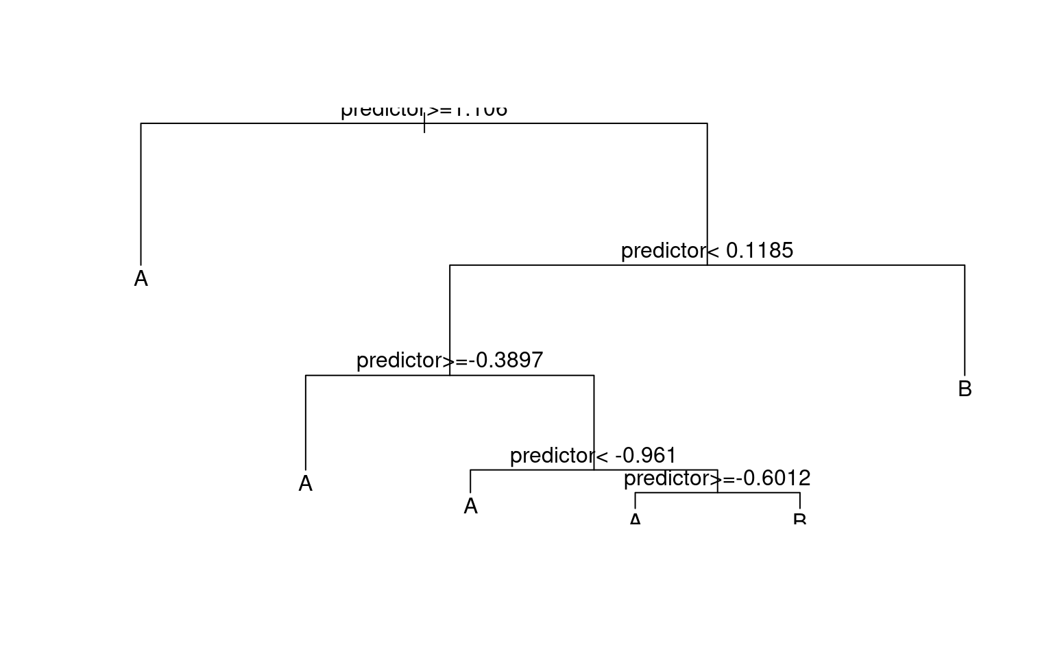
prp(r1)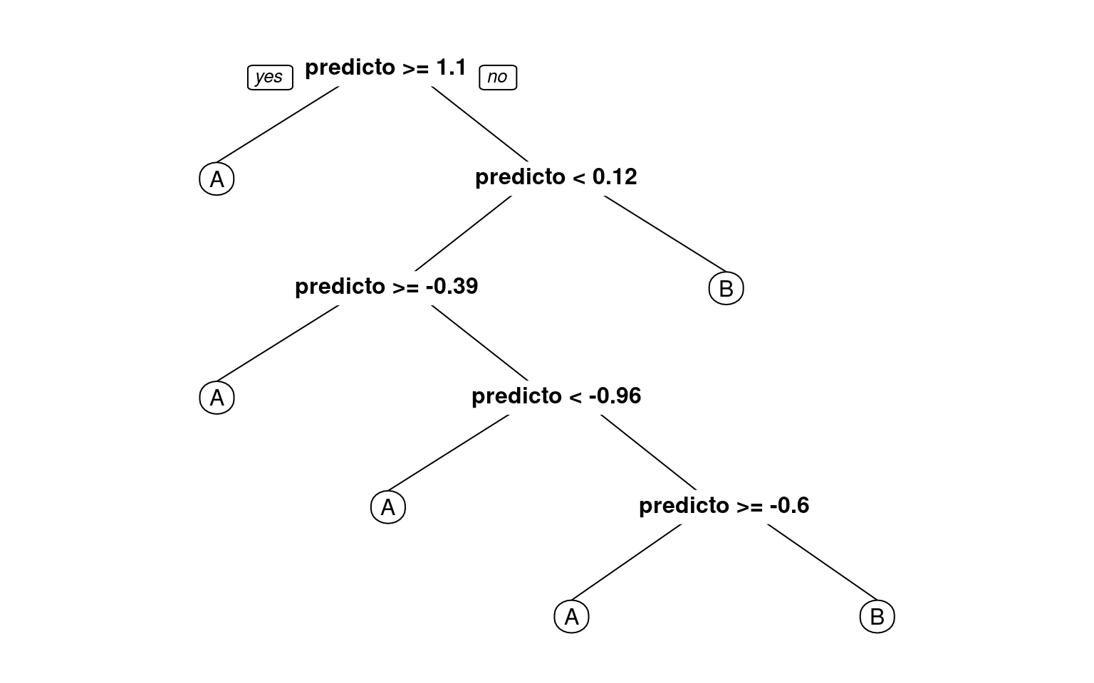
fancyRpartPlot(r1) #better visualization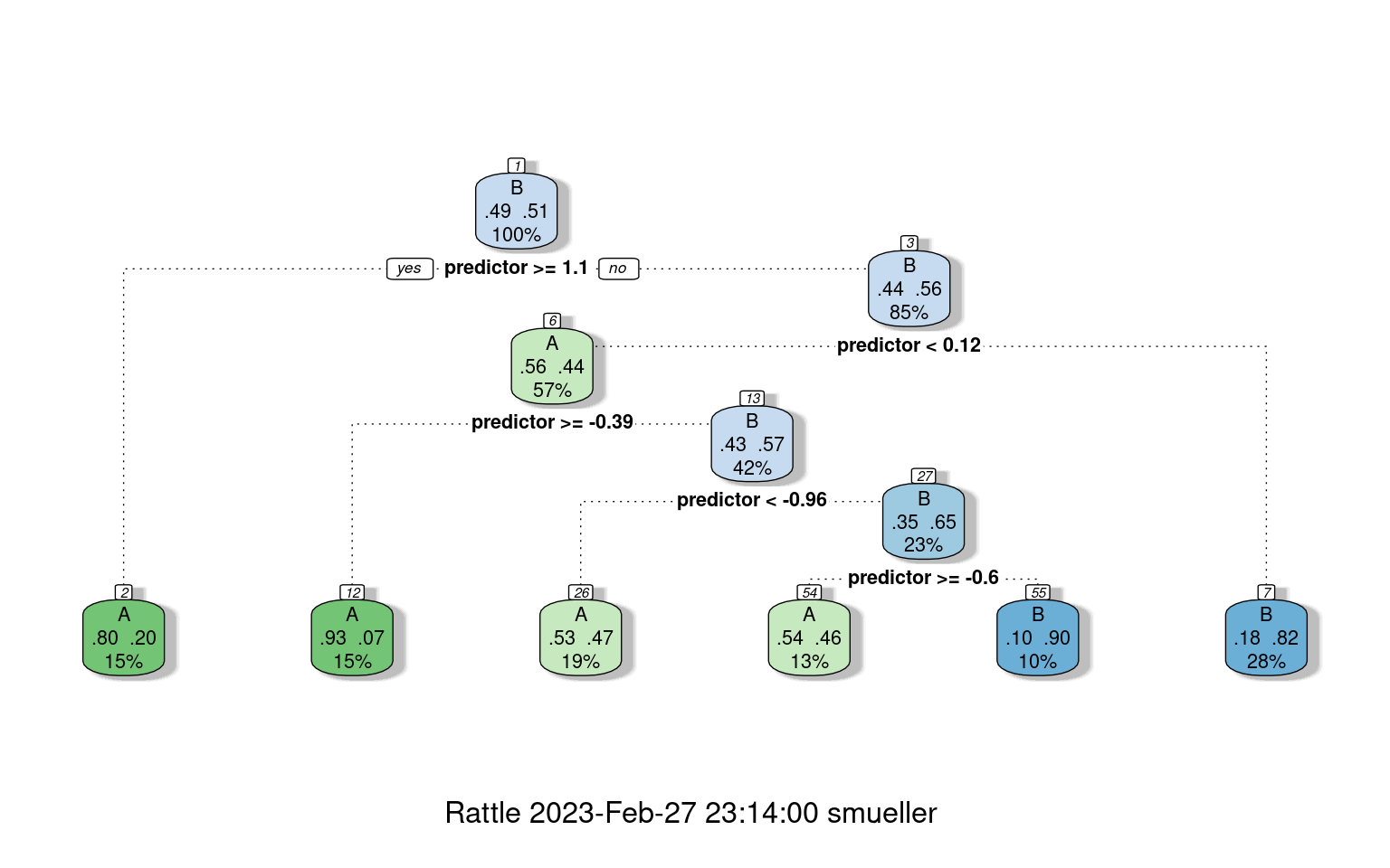
confusion(classes, predict(r1, type = "class"))Overall accuracy = 0.75
Confusion matrix
Predicted (cv)
Actual [,1] [,2]
[1,] 0.878 0.122
[2,] 0.373 0.627plot(predictor, col = factor(classes))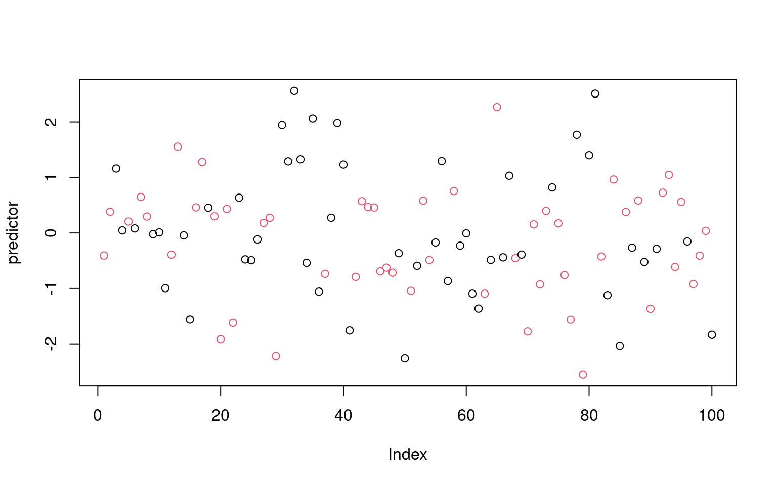 Notice that even though the predictor had no true relationship to the
categories, we were able to get 71% accuracy. We could in fact do
better, just by adding rules. Various aspects of the tree algorithm are
controlled via the control argument, using
Notice that even though the predictor had no true relationship to the
categories, we were able to get 71% accuracy. We could in fact do
better, just by adding rules. Various aspects of the tree algorithm are
controlled via the control argument, using rpart.control.
Here, we set ‘minsplit’ to 1, which says we can split a group as long as
it has at least 1 item. ‘minbucket’ specifies the smallest number of
observations that can appear on the bottom node, and cp is a complexity
argument. It defaults to .01, and is a criterion for how much better
each model must be before splitting a leaf node. A negative value will
mean that any additional node is better, and so it will accept any
split.
r2 <- rpart(classes ~ predictor, method = "class", control = rpart.control(minsplit = 1,
    minbucket = 1, cp = -1))
prp(r2)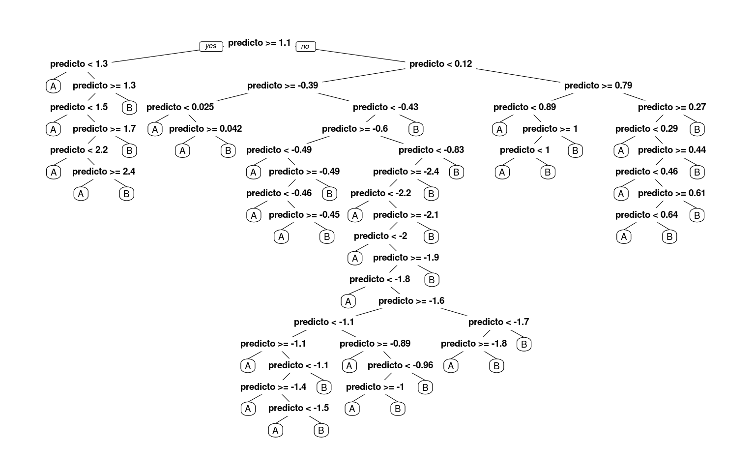
# this tree is a bit too large for this graphics method: fancyRpartPlot(r2)
confusion(classes, predict(r2, type = "class"))
Overall accuracy = 1
Confusion matrix
Predicted (cv)
Actual [,1] [,2]
[1,] 1 0
[2,] 0 1Now, we have completely predicted every item by successively dividing the line. Notice that by default, rpart must choose the best number of nodes to use,, and the default control parameters are set to often be reasonable, but there is no guarantee they are the right ones for your data. This is a critical decision for a decision tree, as it impacts the complexity of the model, and how much it overfits the data.
How will this work for a real data set? Let’s re-load the engineering data set. In this data, we have asked both Engineering and Psychology students to determine whether pairs of words from Psychology, Engineering go together, and measured their time and accuracy.
joint <- read.csv("eng-joint.csv")
joint$eng <- as.factor(c("psych", "eng")[joint$eng + 1])


## This is the partitioning tree:

r1 <- rpart(eng ~ ., data = joint, method = "class")
r1
n= 76
node), split, n, loss, yval, (yprob)
* denotes terminal node
1) root 76 38 eng (0.50000000 0.50000000)
2) ep.1>=2049.256 68 31 eng (0.54411765 0.45588235)
4) ppr.1< 2900.149 39 14 eng (0.64102564 0.35897436)
8) ppr.1>=2656.496 11 1 eng (0.90909091 0.09090909) *
9) ppr.1< 2656.496 28 13 eng (0.53571429 0.46428571)
18) ep>=0.7083333 14 4 eng (0.71428571 0.28571429) *
19) ep< 0.7083333 14 5 psych (0.35714286 0.64285714) *
5) ppr.1>=2900.149 29 12 psych (0.41379310 0.58620690)
10) ppu>=0.8333333 7 2 eng (0.71428571 0.28571429) *
11) ppu< 0.8333333 22 7 psych (0.31818182 0.68181818) *
3) ep.1< 2049.256 8 1 psych (0.12500000 0.87500000) *prp(r1, cex = 0.75)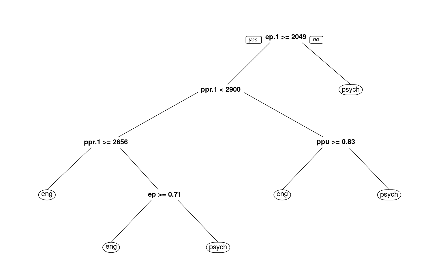
# text(r1,use.n=TRUE)
fancyRpartPlot(r1)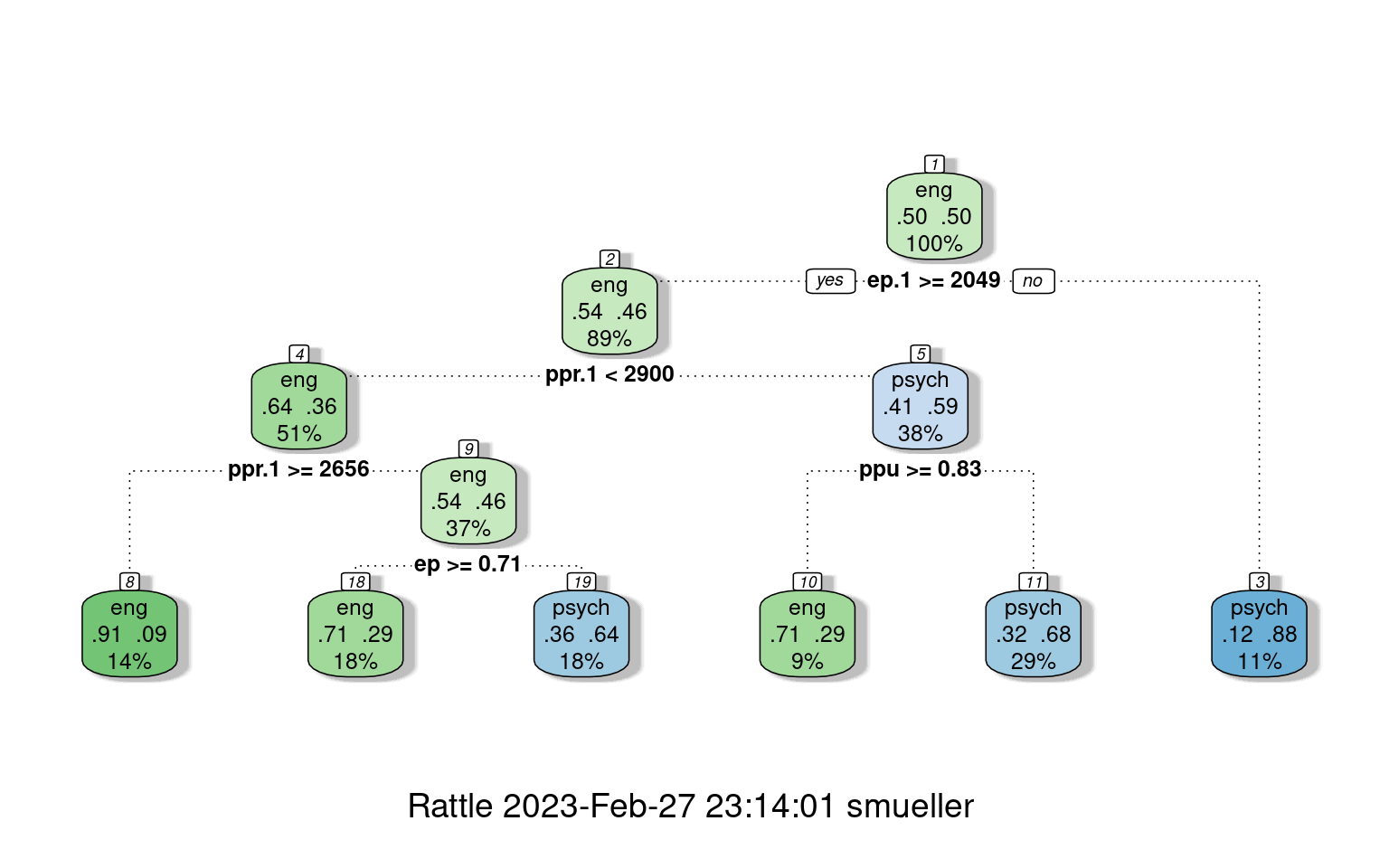
confusion(joint$eng, predict(r1, type = "class"))Overall accuracy = 0.737
Confusion matrix
Predicted (cv)
Actual eng psych
eng 0.658 0.342
psych 0.184 0.816With the default full partitioning, we get 73% accuracy. But the decision tree is fairly complicated. For example, notice that nodes 2 and 4 consecutively select ppr.1 twice. First, if ppr.1 is faster than 2900, it then checks if it is slower than 2656, and makes different decisions based on these narrow ranges of response time. This seems unlikely to be a real or meaningful decision, and we might want something simpler. Let’s only allow it to go to a depth of 2, by controlling maxdepth:
library(rattle)
r2 <- rpart(eng ~ ., data = joint, method = "class", control = rpart.control(maxdepth = 2))
r2
n= 76
node), split, n, loss, yval, (yprob)
* denotes terminal node
1) root 76 38 eng (0.5000000 0.5000000)
2) ep.1>=2049.256 68 31 eng (0.5441176 0.4558824)
4) ppr.1< 2900.149 39 14 eng (0.6410256 0.3589744) *
5) ppr.1>=2900.149 29 12 psych (0.4137931 0.5862069) *
3) ep.1< 2049.256 8 1 psych (0.1250000 0.8750000) *fancyRpartPlot(r2)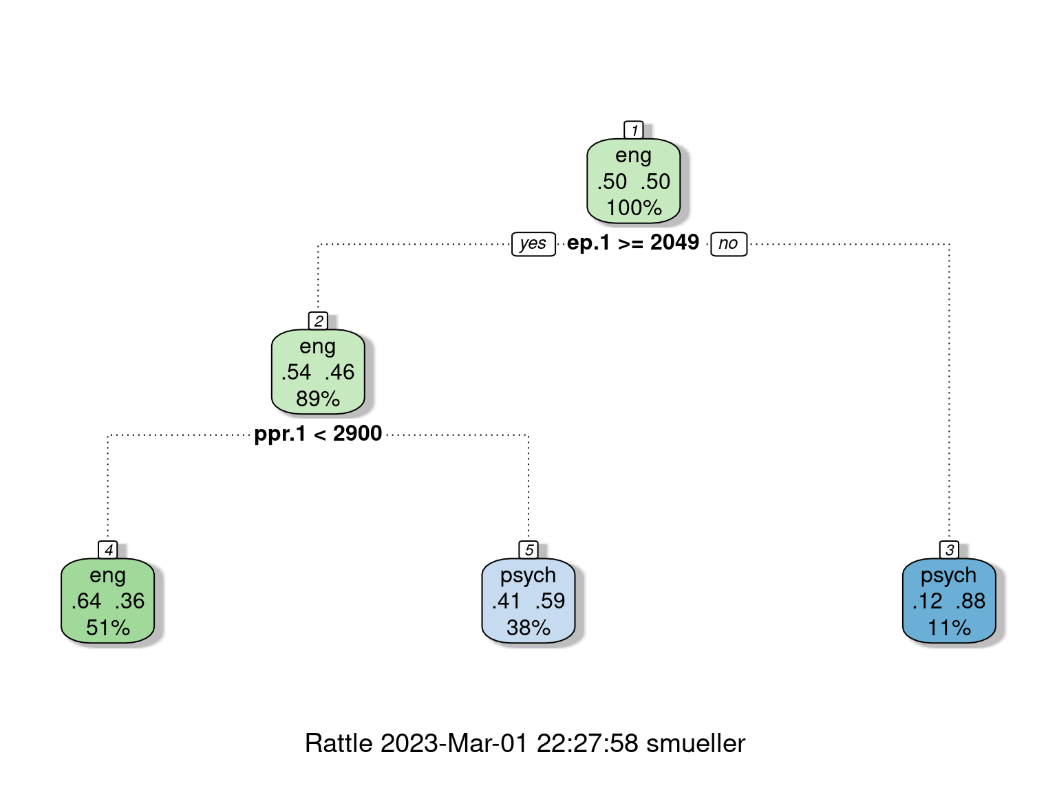
# text(r2,use.n=T)
confusion(joint$eng, predict(r2, type = "class"))
Overall accuracy = 0.645
Confusion matrix
Predicted (cv)
Actual eng psych
eng 0.658 0.342
psych 0.368 0.632Here, we are down to 65% ‘correct’ classifications.
Looking deeper
If we look at the summary of the tree object, it gives us a lot of details about goodness of fit and decision points.
summary(r2)Call:
rpart(formula = eng ~ ., data = joint, method = "class", control = rpart.control(minbucket = 2))
n= 76
CP nsplit rel error xerror xstd
1 0.15789474 0 1.0000000 1.315789 0.1088382
2 0.06140351 1 0.8421053 1.131579 0.1137106
3 0.05263158 8 0.3157895 1.131579 0.1137106
4 0.02631579 9 0.2631579 1.105263 0.1140706
5 0.01000000 13 0.1578947 1.000000 0.1147079
Variable importance
eer.1 ep.1 ppr.1 eeu.1 ppu.1 eeu ep ppr eer
18 17 16 13 11 10 6 5 4
Node number 1: 76 observations, complexity param=0.1578947
predicted class=eng expected loss=0.5 P(node) =1
class counts: 38 38
probabilities: 0.500 0.500
left son=2 (70 obs) right son=3 (6 obs)
Primary splits:
ep.1 < 2017.343 to the right, improve=3.257143, (0 missing)
eeu.1 < 2431.336 to the right, improve=2.326531, (0 missing)
ppr.1 < 5377.582 to the right, improve=2.111111, (0 missing)
ppu.1 < 4579.384 to the right, improve=2.072727, (0 missing)
eer.1 < 4687.518 to the right, improve=1.966874, (0 missing)
Surrogate splits:
eer.1 < 1450.41 to the right, agree=0.947, adj=0.333, (0 split)
eeu.1 < 1693.927 to the right, agree=0.947, adj=0.333, (0 split)
ppu.1 < 1532.392 to the right, agree=0.947, adj=0.333, (0 split)
Node number 2: 70 observations, complexity param=0.06140351
predicted class=eng expected loss=0.4571429 P(node) =0.9210526
class counts: 38 32
probabilities: 0.543 0.457
left son=4 (4 obs) right son=5 (66 obs)
Primary splits:
eer.1 < 1768.284 to the left, improve=1.773160, (0 missing)
ppr.1 < 5377.582 to the right, improve=1.773160, (0 missing)
ppu < 0.8333333 to the right, improve=1.559096, (0 missing)
ppu.1 < 4579.384 to the right, improve=1.542857, (0 missing)
eeu.1 < 6596.24 to the left, improve=1.213445, (0 missing)
Node number 3: 6 observations
predicted class=psych expected loss=0 P(node) =0.07894737
class counts: 0 6
probabilities: 0.000 1.000
Node number 4: 4 observations
predicted class=eng expected loss=0 P(node) =0.05263158
class counts: 4 0
probabilities: 1.000 0.000
Node number 5: 66 observations, complexity param=0.06140351
predicted class=eng expected loss=0.4848485 P(node) =0.8684211
class counts: 34 32
probabilities: 0.515 0.485
left son=10 (4 obs) right son=11 (62 obs)
Primary splits:
ppr.1 < 5377.582 to the right, improve=2.001955, (0 missing)
ppu.1 < 4579.384 to the right, improve=1.912554, (0 missing)
eer.1 < 4687.518 to the right, improve=1.831682, (0 missing)
ppu < 0.8333333 to the right, improve=1.665975, (0 missing)
ep.1 < 5045.675 to the right, improve=1.336364, (0 missing)
Node number 10: 4 observations
predicted class=eng expected loss=0 P(node) =0.05263158
class counts: 4 0
probabilities: 1.000 0.000
Node number 11: 62 observations, complexity param=0.06140351
predicted class=psych expected loss=0.483871 P(node) =0.8157895
class counts: 30 32
probabilities: 0.484 0.516
left son=22 (53 obs) right son=23 (9 obs)
Primary splits:
ppr.1 < 4276.628 to the left, improve=2.9258130, (0 missing)
ppu.1 < 4579.384 to the right, improve=1.8188950, (0 missing)
eer.1 < 7129.535 to the right, improve=1.6796060, (0 missing)
ppu < 0.8333333 to the right, improve=1.3223520, (0 missing)
eeu.1 < 6596.24 to the left, improve=0.9677419, (0 missing)
Surrogate splits:
ep.1 < 5274.203 to the left, agree=0.871, adj=0.111, (0 split)
Node number 22: 53 observations, complexity param=0.06140351
predicted class=eng expected loss=0.4528302 P(node) =0.6973684
class counts: 29 24
probabilities: 0.547 0.453
left son=44 (8 obs) right son=45 (45 obs)
Primary splits:
ppu.1 < 4549.837 to the right, improve=2.0252620, (0 missing)
eer.1 < 4687.518 to the right, improve=1.7743550, (0 missing)
ep.1 < 3637.668 to the right, improve=1.2763460, (0 missing)
ppr < 0.5 to the right, improve=0.9177457, (0 missing)
eeu.1 < 2431.336 to the right, improve=0.9177457, (0 missing)
Surrogate splits:
ppr.1 < 1274.998 to the left, agree=0.906, adj=0.375, (0 split)
eer.1 < 4340.98 to the right, agree=0.887, adj=0.250, (0 split)
ep.1 < 5045.675 to the right, agree=0.887, adj=0.250, (0 split)
eeu.1 < 4075.88 to the right, agree=0.868, adj=0.125, (0 split)
Node number 23: 9 observations
predicted class=psych expected loss=0.1111111 P(node) =0.1184211
class counts: 1 8
probabilities: 0.111 0.889
Node number 44: 8 observations
predicted class=eng expected loss=0.125 P(node) =0.1052632
class counts: 7 1
probabilities: 0.875 0.125
Node number 45: 45 observations, complexity param=0.06140351
predicted class=psych expected loss=0.4888889 P(node) =0.5921053
class counts: 22 23
probabilities: 0.489 0.511
left son=90 (31 obs) right son=91 (14 obs)
Primary splits:
ppr < 0.5 to the right, improve=1.677829, (0 missing)
eer.1 < 2344.133 to the right, improve=1.110511, (0 missing)
ppu.1 < 3962.375 to the left, improve=1.110511, (0 missing)
ppr.1 < 1678.842 to the left, improve=1.093540, (0 missing)
eeu.1 < 2431.336 to the right, improve=1.088889, (0 missing)
Surrogate splits:
eeu.1 < 3750.117 to the left, agree=0.778, adj=0.286, (0 split)
ep < 0.4583333 to the right, agree=0.756, adj=0.214, (0 split)
eer.1 < 2330.756 to the right, agree=0.756, adj=0.214, (0 split)
ep.1 < 3546.093 to the left, agree=0.733, adj=0.143, (0 split)
ppr.1 < 1867.892 to the right, agree=0.711, adj=0.071, (0 split)
Node number 90: 31 observations, complexity param=0.06140351
predicted class=eng expected loss=0.4193548 P(node) =0.4078947
class counts: 18 13
probabilities: 0.581 0.419
left son=180 (15 obs) right son=181 (16 obs)
Primary splits:
eer.1 < 2730.725 to the left, improve=2.7967740, (0 missing)
eeu.1 < 2431.336 to the right, improve=2.3950200, (0 missing)
ppu.1 < 3962.375 to the left, improve=1.7275430, (0 missing)
ppr.1 < 2892.779 to the left, improve=0.9634409, (0 missing)
eer < 0.5 to the left, improve=0.9501075, (0 missing)
Surrogate splits:
ep.1 < 2513.859 to the left, agree=0.710, adj=0.400, (0 split)
ppu.1 < 2662.676 to the left, agree=0.710, adj=0.400, (0 split)
eeu.1 < 2866.971 to the left, agree=0.677, adj=0.333, (0 split)
ppr.1 < 2824.401 to the left, agree=0.677, adj=0.333, (0 split)
eer < 0.5 to the left, agree=0.645, adj=0.267, (0 split)
Node number 91: 14 observations, complexity param=0.02631579
predicted class=psych expected loss=0.2857143 P(node) =0.1842105
class counts: 4 10
probabilities: 0.286 0.714
left son=182 (9 obs) right son=183 (5 obs)
Primary splits:
eeu < 0.5 to the right, improve=1.269841, (0 missing)
eer.1 < 2416.786 to the right, improve=1.269841, (0 missing)
ep < 0.4583333 to the left, improve=1.108225, (0 missing)
ep.1 < 3903.651 to the right, improve=1.108225, (0 missing)
ppr.1 < 3215.113 to the right, improve=1.108225, (0 missing)
Surrogate splits:
ep < 0.8333333 to the left, agree=0.786, adj=0.4, (0 split)
eeu.1 < 2589.253 to the right, agree=0.786, adj=0.4, (0 split)
ep.1 < 2231.651 to the right, agree=0.786, adj=0.4, (0 split)
ppr < 0.1666667 to the right, agree=0.714, adj=0.2, (0 split)
ppu < 0.5 to the right, agree=0.714, adj=0.2, (0 split)
Node number 180: 15 observations, complexity param=0.02631579
predicted class=eng expected loss=0.2 P(node) =0.1973684
class counts: 12 3
probabilities: 0.800 0.200
left son=360 (8 obs) right son=361 (7 obs)
Primary splits:
eeu.1 < 2431.631 to the right, improve=1.3714290, (0 missing)
eeu < 0.5 to the right, improve=0.9818182, (0 missing)
eer.1 < 2515.267 to the right, improve=0.8000000, (0 missing)
ppu.1 < 2570.591 to the right, improve=0.8000000, (0 missing)
ep.1 < 2406.521 to the left, improve=0.6000000, (0 missing)
Surrogate splits:
ep.1 < 2465.887 to the right, agree=0.733, adj=0.429, (0 split)
eeu < 0.5 to the right, agree=0.667, adj=0.286, (0 split)
eer.1 < 2528.369 to the right, agree=0.667, adj=0.286, (0 split)
ppu.1 < 1856.145 to the right, agree=0.667, adj=0.286, (0 split)
ep < 0.5416667 to the left, agree=0.600, adj=0.143, (0 split)
Node number 181: 16 observations, complexity param=0.06140351
predicted class=psych expected loss=0.375 P(node) =0.2105263
class counts: 6 10
probabilities: 0.375 0.625
left son=362 (7 obs) right son=363 (9 obs)
Primary splits:
eeu < 0.5 to the left, improve=2.8650790, (0 missing)
eeu.1 < 2431.336 to the right, improve=2.0454550, (0 missing)
eer.1 < 3816.402 to the right, improve=1.7857140, (0 missing)
ep.1 < 2578.796 to the right, improve=1.0384620, (0 missing)
ppr < 0.8333333 to the left, improve=0.8333333, (0 missing)
Surrogate splits:
eer < 0.8333333 to the right, agree=0.688, adj=0.286, (0 split)
ppr < 0.8333333 to the left, agree=0.688, adj=0.286, (0 split)
eer.1 < 3816.402 to the right, agree=0.688, adj=0.286, (0 split)
ep.1 < 3322.808 to the right, agree=0.688, adj=0.286, (0 split)
ppr.1 < 3660.362 to the right, agree=0.688, adj=0.286, (0 split)
Node number 182: 9 observations, complexity param=0.02631579
predicted class=psych expected loss=0.4444444 P(node) =0.1184211
class counts: 4 5
probabilities: 0.444 0.556
left son=364 (2 obs) right son=365 (7 obs)
Primary splits:
ep < 0.4583333 to the left, improve=1.587302, (0 missing)
ep.1 < 3903.651 to the right, improve=1.587302, (0 missing)
ppr.1 < 3215.113 to the right, improve=1.587302, (0 missing)
eer.1 < 2387.215 to the right, improve=1.015873, (0 missing)
ppu.1 < 2349.516 to the right, improve=1.015873, (0 missing)
Surrogate splits:
ppr.1 < 3215.113 to the right, agree=1, adj=1, (0 split)
Node number 183: 5 observations
predicted class=psych expected loss=0 P(node) =0.06578947
class counts: 0 5
probabilities: 0.000 1.000
Node number 360: 8 observations
predicted class=eng expected loss=0 P(node) =0.1052632
class counts: 8 0
probabilities: 1.000 0.000
Node number 361: 7 observations, complexity param=0.02631579
predicted class=eng expected loss=0.4285714 P(node) =0.09210526
class counts: 4 3
probabilities: 0.571 0.429
left son=722 (3 obs) right son=723 (4 obs)
Primary splits:
ep.1 < 2385.735 to the left, improve=1.9285710, (0 missing)
eeu.1 < 2369.62 to the left, improve=1.8285710, (0 missing)
eer.1 < 2515.267 to the right, improve=1.0285710, (0 missing)
ppu.1 < 1929.897 to the left, improve=1.0285710, (0 missing)
eeu < 0.5 to the right, improve=0.5952381, (0 missing)
Surrogate splits:
eeu < 0.5 to the right, agree=0.857, adj=0.667, (0 split)
ppu.1 < 2576.52 to the right, agree=0.857, adj=0.667, (0 split)
eer < 0.8333333 to the left, agree=0.714, adj=0.333, (0 split)
ep < 0.7083333 to the left, agree=0.714, adj=0.333, (0 split)
eer.1 < 2465.266 to the left, agree=0.714, adj=0.333, (0 split)
Node number 362: 7 observations, complexity param=0.05263158
predicted class=eng expected loss=0.2857143 P(node) =0.09210526
class counts: 5 2
probabilities: 0.714 0.286
left son=724 (5 obs) right son=725 (2 obs)
Primary splits:
eeu.1 < 2431.336 to the right, improve=2.8571430, (0 missing)
eer.1 < 3282.949 to the right, improve=1.5238100, (0 missing)
ppu < 0.8333333 to the right, improve=0.8571429, (0 missing)
ep < 0.7083333 to the left, improve=0.4571429, (0 missing)
ep.1 < 3435.295 to the right, improve=0.4571429, (0 missing)
Surrogate splits:
eer.1 < 3282.949 to the right, agree=0.857, adj=0.5, (0 split)
Node number 363: 9 observations
predicted class=psych expected loss=0.1111111 P(node) =0.1184211
class counts: 1 8
probabilities: 0.111 0.889
Node number 364: 2 observations
predicted class=eng expected loss=0 P(node) =0.02631579
class counts: 2 0
probabilities: 1.000 0.000
Node number 365: 7 observations
predicted class=psych expected loss=0.2857143 P(node) =0.09210526
class counts: 2 5
probabilities: 0.286 0.714
Node number 722: 3 observations
predicted class=eng expected loss=0 P(node) =0.03947368
class counts: 3 0
probabilities: 1.000 0.000
Node number 723: 4 observations
predicted class=psych expected loss=0.25 P(node) =0.05263158
class counts: 1 3
probabilities: 0.250 0.750
Node number 724: 5 observations
predicted class=eng expected loss=0 P(node) =0.06578947
class counts: 5 0
probabilities: 1.000 0.000
Node number 725: 2 observations
predicted class=psych expected loss=0 P(node) =0.02631579
class counts: 0 2
probabilities: 0.000 1.000 This model seems to fit a lot better than our earlier LDA models, which suggest that it is probably overfitting. Cross-validation can be done within the control parameter \(xval\):
r3 <- rpart(eng ~ ., data = joint, method = "class", control = c(maxdepth = 3, xval = 10))
r3
n= 76
node), split, n, loss, yval, (yprob)
* denotes terminal node
1) root 76 38 eng (0.5000000 0.5000000)
2) ep.1>=2049.256 68 31 eng (0.5441176 0.4558824)
4) ppr.1< 2900.149 39 14 eng (0.6410256 0.3589744) *
5) ppr.1>=2900.149 29 12 psych (0.4137931 0.5862069)
10) ppu>=0.8333333 7 2 eng (0.7142857 0.2857143) *
11) ppu< 0.8333333 22 7 psych (0.3181818 0.6818182) *
3) ep.1< 2049.256 8 1 psych (0.1250000 0.8750000) *confusion(joint$eng, predict(r1, type = "class"))Overall accuracy = 0.737
Confusion matrix
Predicted (cv)
Actual eng psych
eng 0.658 0.342
psych 0.184 0.816confusion(joint$eng, predict(r3, type = "class"))Overall accuracy = 0.684
Confusion matrix
Predicted (cv)
Actual eng psych
eng 0.789 0.211
psych 0.421 0.579Accuracy goes down a bit, but the 74% accuracy is about what we achieved in the simple lda models.
Clearly, for partitioning trees, we have to be careful about overfitting, because we can always easily get the perfect classification.
Regression Trees
Instead of using a tree to divide and predict group memberships, rpart can also use a tree as a sort of regression. It tries to model all of the data within a group as a single intercept value, and then tries to divide groups to improve fit. There are some pdf help files available for more detail, but the regression options (including poisson and anova) are a bit poorly documented. But, basically, we can use the same ideas to partition the data, and then fit either a single value within each group or some small linear model. The tree shows nodes with the the top value the mean for that branch.
cw <- rpart(weight ~ Time + Diet, data = ChickWeight, control = rpart.control(maxdepth = 5))
summary(cw)
Call:
rpart(formula = weight ~ Time + Diet, data = ChickWeight, control = rpart.control(maxdepth = 5))
n= 578
CP nsplit rel error xerror xstd
1 0.54964983 0 1.0000000 1.0063862 0.06435131
2 0.08477800 1 0.4503502 0.4759351 0.03696654
3 0.04291979 2 0.3655722 0.3878498 0.02995419
4 0.03905827 3 0.3226524 0.3538543 0.02969765
5 0.01431308 4 0.2835941 0.3102103 0.02746108
6 0.01000000 5 0.2692810 0.3020699 0.02757267
Variable importance
Time Diet
93 7
Node number 1: 578 observations, complexity param=0.5496498
mean=121.8183, MSE=5042.484
left son=2 (296 obs) right son=3 (282 obs)
Primary splits:
Time < 11 to the left, improve=0.54964980, (0 missing)
Diet splits as LRRR, improve=0.04479917, (0 missing)
Node number 2: 296 observations, complexity param=0.04291979
mean=70.43243, MSE=700.6779
left son=4 (149 obs) right son=5 (147 obs)
Primary splits:
Time < 5 to the left, improve=0.60314240, (0 missing)
Diet splits as LRRR, improve=0.04085943, (0 missing)
Node number 3: 282 observations, complexity param=0.084778
mean=175.7553, MSE=3919.043
left son=6 (144 obs) right son=7 (138 obs)
Primary splits:
Time < 17 to the left, improve=0.2235767, (0 missing)
Diet splits as LLRR, improve=0.1333256, (0 missing)
Node number 4: 149 observations
mean=50.01342, MSE=71.0468
Node number 5: 147 observations
mean=91.12925, MSE=487.9085
Node number 6: 144 observations, complexity param=0.01431308
mean=146.7778, MSE=1825.326
left son=12 (84 obs) right son=13 (60 obs)
Primary splits:
Diet splits as LLRR, improve=0.1587094, (0 missing)
Time < 15 to the left, improve=0.1205157, (0 missing)
Node number 7: 138 observations, complexity param=0.03905827
mean=205.9928, MSE=4313.283
left son=14 (80 obs) right son=15 (58 obs)
Primary splits:
Diet splits as LLRR, improve=0.19124870, (0 missing)
Time < 19 to the left, improve=0.02989732, (0 missing)
Node number 12: 84 observations
mean=132.3929, MSE=1862.834
Node number 13: 60 observations
mean=166.9167, MSE=1077.543
Node number 14: 80 observations
mean=181.5375, MSE=3790.849
Node number 15: 58 observations
mean=239.7241, MSE=3071.165 fancyRpartPlot(cw)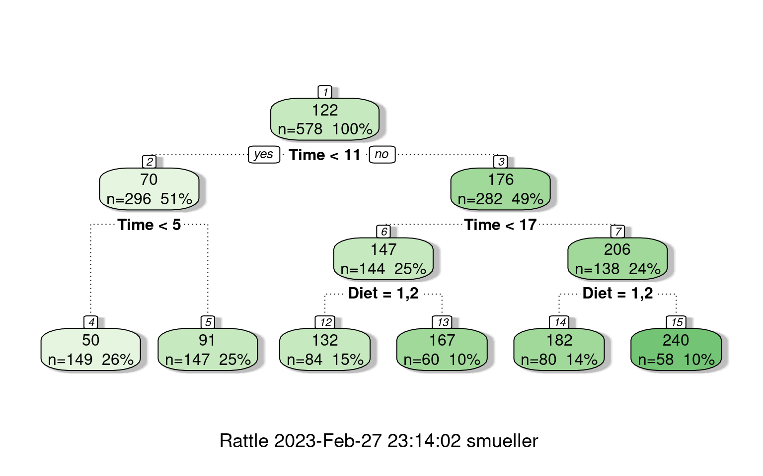
## this shows the yvalue estimate for each leaf node:
cw$frame
var n wt dev yval complexity ncompete nsurrogate
1 Time 578 578 2914555.93 121.81834 0.549649827 1 0
2 Time 296 296 207400.65 70.43243 0.042919791 1 0
4 <leaf> 149 149 10585.97 50.01342 0.010000000 0 0
5 <leaf> 147 147 71722.54 91.12925 0.007137211 0 0
3 Time 282 282 1105170.12 175.75532 0.084778005 1 0
6 Diet 144 144 262846.89 146.77778 0.014313079 1 0
12 <leaf> 84 84 156478.04 132.39286 0.005288100 0 0
13 <leaf> 60 60 64652.58 166.91667 0.005342978 0 0
7 Diet 138 138 595232.99 205.99275 0.039058272 1 0
[ reached 'max' / getOption("max.print") -- omitted 2 rows ]library(ggplot2)
ChickWeight$predicted <- predict(cw)
ggplot(ChickWeight, aes(x = Time, y = predicted, group = Diet, color = Diet, size = Diet)) +
geom_point(shape = 1) + theme_minimal()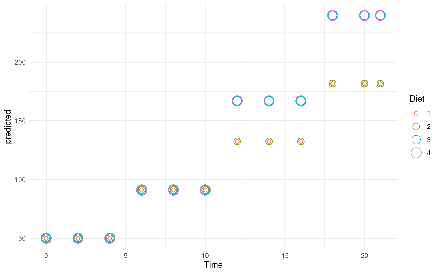 # Random Forests
One advantage of partitioning/decision trees is that they are fast and easy to make. They are also considered interpretable and easy to understand. A tree like this can be used by a doctor or a medical counselor to help understand the risk for a disease, by asking a few simple questions.
The downsides of a decision tree is that they are often not very good, especially once they have been trimmed to avoid over-fitting. Recently, researchers have been interested in combining the results of many small (and often not-very-good) classifiers to make one better one. This often is described as ‘boosting’, or `ensemble’ methods, and there are a number of ways to achieve this. Doing this in a particular way with decision trees is referred to as a ‘random forest’ (see Breiman and Cutler).
Random forests can be used for both regression and classification (trees can be used in either way as well), and the classification and regression trees (CART) approach is a method that supports both. A random forest works as follows:
- Build \(N\) trees (where N may be hundreds; Brieman says ‘Don’t be stingy’), where each tree is built from a random subset of features/variables. That is, on each step, choose the best variable to divide the branch based on a random subset of variables.
For each tree: 1. Pick a random sample of data. This is by default ‘bootstrapped’, meaning it has the same size as your data but samples it with replacement. 2. Pick K, where k is the number of variables considered at each step (typically sqrt(number of variables)) 3. Select k variables at random. 4. Find the best split among those k variables. 5. Repeat from point 3 until you reach the end criteria (determined by maxnodes and nodesize)
- Then, to classify your data, have each tree determine its best guess, and then take the most frequent outcome (or give a probabilistic answer based on the balance of evidence). This can both provide a robust classifier and a general importance of variables. You can look at the trees that more more accurate and see which variables were used, and which were used earlier, and this can give an indication of the most robust classification. In contrast to a normal CART, where the first cut may end up not being as important as later cuts.
The randomForest package in R supports building these models. Because these can be a bit more difficult to comprehend, there is a companion package randomForestExplainer that is also handy in digging down on the types of forests derived.
library(randomForest)
library(randomForestExplainer)

rf <- randomForest(x = joint[, -1], y = joint$eng, proximity = T, ntree = 5000)
rf
Call:
 randomForest(x = joint[, -1], y = joint$eng, ntree = 5000, proximity = T)
               Type of random forest: classification
                     Number of trees: 5000
No. of variables tried at each split: 3

        OOB estimate of  error rate: 55.26%
Confusion matrix:
      eng psych class.error
eng    17    21   0.5526316
psych  21    17   0.5526316
# printRandomForests(rf) ##look at all the RFs
confusion(joint$eng, predict(rf))Overall accuracy = 0.447
Confusion matrix
Predicted (cv)
Actual eng psych
eng 0.447 0.553
psych 0.553 0.447If you run this repeatedly, you get a different answer each time. For this data, quite often the accuracy is below chance. The confusion matrix produced is “OOB”: out-of-bag, which is like Leave-on-out cross-validation. Looking at the trees, they are quite complex as well, with tens of rules. We can get a printout of individual subtrees with getTree:
(getTree(rf, 1)) left daughter right daughter split var split point status prediction
1 2 3 7 2431.3361678 1 0
2 4 5 4 0.8333333 1 0
3 6 7 4 0.5000000 1 0
4 8 9 5 0.5000000 1 0
5 10 11 10 1812.9655820 1 0
6 12 13 6 3531.3683056 1 0
7 14 15 1 0.5000000 1 0
8 16 17 9 1758.7191269 1 0
9 18 19 2 0.5000000 1 0
10 0 0 0 0.0000000 -1 2
11 0 0 0 0.0000000 -1 1
12 20 21 9 2466.8956962 1 0
[ reached getOption("max.print") -- omitted 31 rows ](getTree(rf, 5)) left daughter right daughter split var split point status prediction
1 2 3 3 0.7916667 1 0
2 4 5 6 1768.2841289 1 0
3 6 7 2 0.8333333 1 0
4 0 0 0 0.0000000 -1 1
5 8 9 9 5377.5822550 1 0
6 10 11 3 0.9583333 1 0
7 0 0 0 0.0000000 -1 1
8 12 13 6 4676.3325617 1 0
9 0 0 0 0.0000000 -1 1
10 14 15 5 0.5000000 1 0
11 0 0 0 0.0000000 -1 2
12 16 17 2 0.5000000 1 0
[ reached getOption("max.print") -- omitted 27 rows ]There are many arguments that support the sampling/evaluation process. The feasibility of changing these will often depend on the size of the data set. With a large data set and many variables, fitting one of these models may take a long time if they are not constrained. Here we look at:
- sampsize: number of bootstrapped samples to try.
- replace: bootstrapped cases are sampled with or without replacement
- mtry: how many variables to try at each split
- ntree: how many trees to grow
- keep.inbag: keep track of which samples are ‘in the bag’
rf <- randomForest(eng ~ ., data = joint, proximity = T, replace = F, mtry = 3, maxnodes = 5,
    ntree = 500, keep.inbag = T, sampsize = 10, localImp = TRUE)

confusion(joint$eng, predict(rf))
Overall accuracy = 0.474
Confusion matrix
Predicted (cv)
Actual eng psych
eng 0.421 0.579
psych 0.474 0.526The forest lets us understand which variables are more important, by identifying how often variables are closer to the root of the tree. Depending on the run, these figures change, but a variable that is frequently selected as the root, or one whose mean depth is low, is likely to be more important.
plot_min_depth_distribution(rf)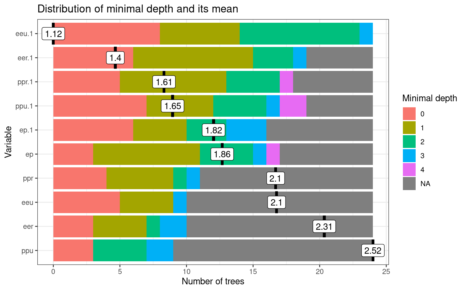
plot_multi_way_importance(rf)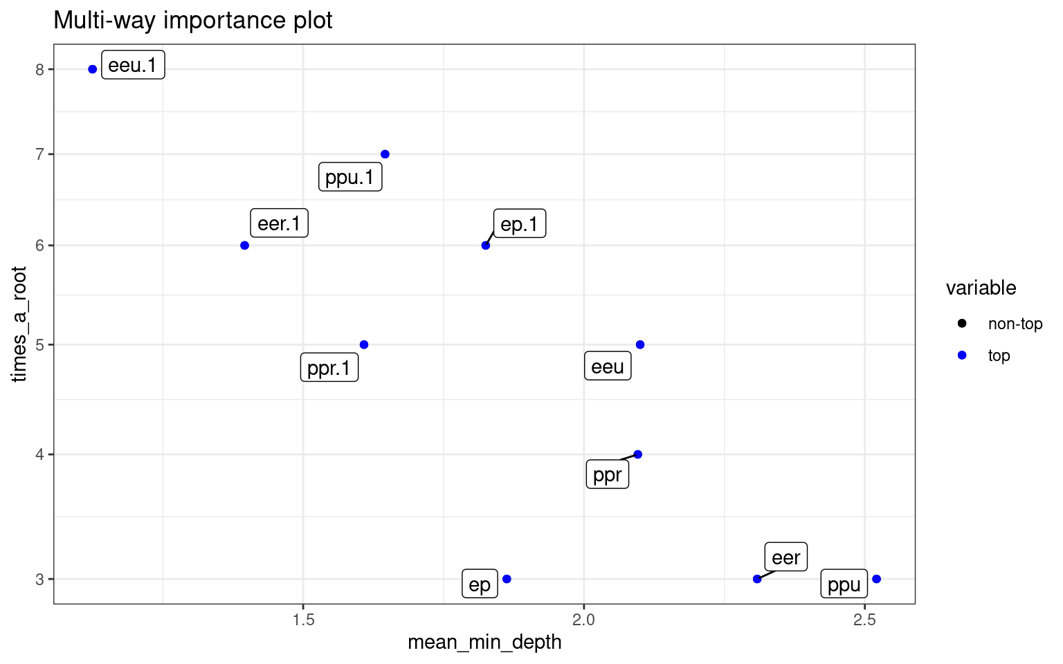
This plots the prediction of the forest for different values of variables. If the variables are useful, we will tend to see blocks of red/purple indicating the prediction in different regions.:
plot_predict_interaction(rf, joint, "eer", "ppr")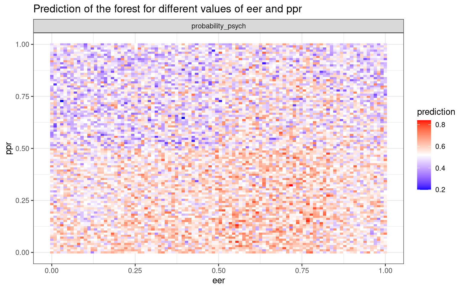
Note that the random forest rarely produces a good classification for the engineers/psychologist data. How does it doe for the iphone data?
phone <- read.csv("data_study1.csv")
phone.dt <- rpart(Smartphone ~ ., data = phone)
prp(phone.dt, cex = 0.5)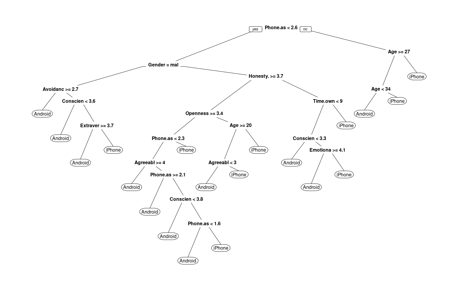
confusion(phone$Smartphone, predict(phone.dt)[, 1] < 0.5)Overall accuracy = 0.783
Confusion matrix
Predicted (cv)
Actual [,1] [,2]
[1,] 0.658 0.342
[2,] 0.129 0.871## this doesn't like the predicted value to be a factor phone$Smartphone<-
## phone$Smartphone=='iPhone' newer versions require this to be a factor:
phone$Smartphone <- as.factor(phone$Smartphone)phone.rf <- randomForest(Smartphone ~ ., data = phone)
phone.rf
Call:
 randomForest(formula = Smartphone ~ ., data = phone)
               Type of random forest: classification
                     Number of trees: 500
No. of variables tried at each split: 3

        OOB estimate of  error rate: 35.16%
Confusion matrix:
        Android iPhone class.error
Android     106    113   0.5159817
iPhone 73 237 0.2354839confusion(phone$Smartphone, predict(phone.rf))Overall accuracy = 0.648
Confusion matrix
Predicted (cv)
Actual Android iPhone
Android 0.484 0.516
iPhone 0.235 0.765This does not seem to be better than the other models for the iphone data, but at least it is comparable. It does not seem to do as well as rpart though!
Note the ranger library random forest gives roughly
equivalent results.
library(ranger)
r2 <- ranger(Smartphone ~ ., data = phone)
r2
Ranger result
Call:
ranger(Smartphone ~ ., data = phone)
Type: Classification
Number of trees: 500
Sample size: 529
Number of independent variables: 12
Mtry: 3
Target node size: 1
Variable importance mode: none
Splitrule: gini
OOB prediction error: 36.29 % treeInfo(r2) nodeID leftChild rightChild splitvarID splitvarName splitval terminal
1 0 1 2 1 Age 22.50 FALSE
2 1 3 4 2 Honesty.Humility 3.15 FALSE
3 2 5 6 2 Honesty.Humility 2.65 FALSE
4 3 7 8 2 Honesty.Humility 1.75 FALSE
5 4 9 10 0 Gender 1.50 FALSE
6 5 11 12 8 Avoidance.Similarity 3.25 FALSE
7 6 13 14 5 Agreeableness 3.25 FALSE
8 7 15 16 8 Avoidance.Similarity 1.65 FALSE
9 8 17 18 3 Emotionality 4.25 FALSE
prediction
1 <NA>
2 <NA>
3 <NA>
4 <NA>
5 <NA>
6 <NA>
7 <NA>
8 <NA>
9 <NA>
[ reached 'max' / getOption("max.print") -- omitted 228 rows ]confusion(phone$Smartphone, predictions(r2))Overall accuracy = 0.637
Confusion matrix
Predicted (cv)
Actual Android iPhone
Android 0.452 0.548
iPhone 0.232 0.768For the examples we looked at, random forests did not perform that well. However, for large complex classifications they can both be more sensitive and provide more convincing explanations than trees, because they can give probabilistic and importance weightings to each variable. However, they do lose some of the simplicity and as we saw, don’t always improve performance of the classifier.
K Nearest-Neighbor classifiers
Another non-model-based classifier are nearest-neighbor methods. These methods require you to develop a similarity or distance space–usually on the basis of a set of predictors or features. Once this distance space is defined, we determine the class by finding the nearest neighbor in that space, and using that label. Because this could be susceptible to noisy data, we usually find a set of \(k\) neighbors and have them vote on the outcome. These are K-nearest neighbor classifiers, or KNN.
Choosing K.
The choice of \(k\) can have a big impact on the results. If \(k\) is too small, classification will be highly impacted by local neighborhood; if it is too big (i.e., if K = N), it will always just respond with the most likely response in the entire population.
Distance Metric
The distance metric used in KNN easily be chosen poorly. For example, if you want to decide on political party based on age, income level, and gender, you need to figure out how to weigh and combine these. By default, you might add differences along each dimension, which would combine something that differs on the scale of dozens with something that differs on the scale of thousands, and so the KNN model would essentially ignore gender and age.
Normalization selection
A typical approach would be to normalize all variables first. Then each variable has equal weight and range.
Using KNN
Unlike previous methods where we train a system based on data and then make classifications, for KNN the trained system is just the data.
Libraries and functions.
There are several options for knn classifers. ### Library: Class * Function: knn * Function: knn.cv (cross-validation)
Library: kknn
- Function: kknn
This provides a ‘weighted k-nearest neighbor classifier’. Here, weighting is a weighting kernel, which gives greater weights to the nearer neighbors.
Library: klaR
- Function: sknn A ‘simple’ knn function. Permits using a weighting kernel as well.
Function: nm
This provides a ‘nearest mean’ classifier
Example
In general, we need to normalize the variables first when using knn, because it tries to create a distance metric between cases–we don’t want distance to be dominated by a variable that happens to have a larger scale.
phone <- read.csv("data_study1.csv")
# Normalizing the values by creating a new function
normal = function(x) {
xn = (x - min(x))/(max(x) - min(x))
return(xn)
}
phone2 <- phone
phone2$Gender <- as.numeric(as.factor(phone2$Gender))
for (i in 2:ncol(phone2)) {
phone2[, i] = normal(as.numeric(phone2[, i]))
}
# we might also use scale:
phone3 <- scale(phone[, -(1:2)])
# checking the range of values after normalization
par(mfrow = c(3, 1))
boxplot(phone[, 3:12])
boxplot(phone2[, 3:12])
boxplot(phone3)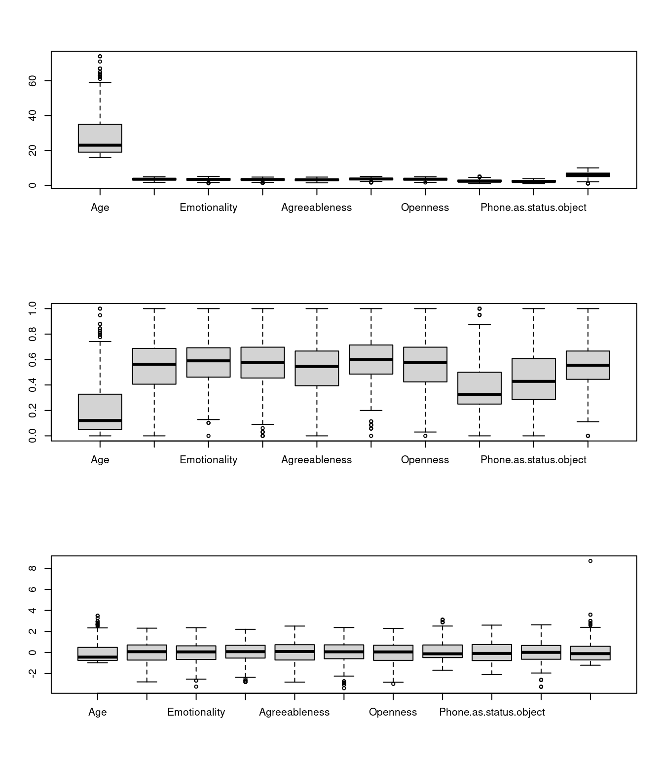 ## Fitting a simple KNN model
Here, we use the class:knn model. We specify separate the training and testing separately, but they can be the same. ‘training’ a knn is a bit deceptive, the training pool is just the set of points being used to classify the test cases. We will use a k of 11, which means each case will be compared to the 11 closes cases and a decision made based on the vote of those. Using an odd number means that there won’t be a tie.
library(class)
m1 = knn(train = phone2[, -1], test = phone2[, -1], cl = phone2$Smartphone, k = 11)
confusion(phone2$Smartphone, m1)
Overall accuracy = 0.688
Confusion matrix
Predicted (cv)
Actual [,1] [,2]
[1,] 0.557 0.443
[2,] 0.219 0.781That is pretty good, but what if we expand k
m1 = knn(train = phone2[, -1], test = phone2[, -1], cl = phone2$Smartphone, k = 25)
confusion(phone2$Smartphone, m1)
Overall accuracy = 0.686
Confusion matrix
Predicted (cv)
Actual [,1] [,2]
[1,] 0.534 0.466
[2,] 0.206 0.794It looks we the choice of k is not going to matter much. What we could do is play with cross-validation though–right now we are testing on the same set as we are ‘training’ with, which will boost our accuracy (since the correct answer will always be one of the elements.) We can also try to do variable selection to change the similarity space to something that works better.
phone2 <- phone2[order(runif(nrow(phone2))), ]  #random sort
phone.train = phone2[1:450, 2:12]
phone.test = phone2[451:nrow(phone2), 2:12]
phone.train.target = phone2[1:450, 1]
phone.test.target = phone2[451:nrow(phone2), 1]

train <- sample(1:nrow(phone2), 300)
m2 <- knn(train = phone.train, test = phone.test, cl = phone.train.target, k = 10)
confusion(phone.test.target, m2)
Overall accuracy = 0.557
Confusion matrix
Predicted (cv)
Actual [,1] [,2]
[1,] 0.567 0.433
[2,] 0.449 0.551Additional resources
K-Nearest Neighbor Classification:
- MASS: Chapter 12.3, p. 341
- https://rstudio-pubs-static.s3.amazonaws.com/123438_3b9052ed40ec4cd2854b72d1aa154df9.html
Relevant library/functions in R:
Decision Trees:
- Faraway, Chapter 13
Library: rpart (function rpart)
Random Forest Classification:
References: - https://www.r-bloggers.com/predicting-wine-quality-using-random-forests/ - https://www.stat.berkeley.edu/~breiman/RandomForests/ - Library: randomForest (Function randomForest) - ranger (a fast random forest implementation).