Support Vector Machines

Support vector machines

The classification methods we have discussed so far can do well for data analytics, with relatively few predictors, when clarity and transparency are needed. As the goal gets more complex, features get less transparent and less interpretable, the number of examples get large, and number of classes get large, these properties will sometimes take a backseat to performance.

LDA and QDA have some limitations. They ASSUME normality, and compute the multi-dimensional mean of each group, form a discriminant function on the line between means, and use a linear or quadratic decision criterion orthogonal to that line. But what if the points are not normal? If the point clouds take on strange shapes, this might not be the right approach. What was critical in the first place was a criterion plane (or quadratic surface) that distinguishes the two groups.

A more sophisticated method tries to find that criterion plane by other means. The algorithm called a ‘support vector machine’ is the most well-known, and is also called a ‘kernel’ methods. In general, they are suitable for complex problems with relatively large training sets, and they rose to popularity following the limitations of early neural network models.

Some of these methods become a challenge as complexity scales large. These include: * Optimization. The least-squares approach used in regression, and maximum likelihood methods used in the glm may not scale well as the number of predictors get large. SVMs typically attempt to map the problem into a problem referred to as a ‘quadratic programming’ (QP) problem, which uses numerical methods to optimize the multi-variate function.

Complex Features. For some types of data (such as audio, imagery, and video), we might be interested in creating complex features and use simple methods to classify. For example, to classify written text, we might identify lines in certain angles and combinations of these lines. To identify speech, we might try to translate into phonemes and then into sound patterns, and finally to words. In contrast, SVMs use what is referred to as a kernel–a way of measuring the similarity between any two exemplars. When a well-understood kernel is used, this permits substantial more efficiency. Furthermore, the useful features may be complex combinations or transformations of the raw features, which a kernel may make easier to manage.
Decision bounds. For simple classifications, decision rules based on simple combinations of features were sufficient. As the exemplar space gets complex, the bounds will become non-linear. Rather than choosing a simple bound based on maximizing cross-validation accuracy, a decision boundary and appropriate transformations are chosen that maximize the gap between groups (while minimizing mis-classification). These transformations can include, essentially, automatically examining interactions between features and using polynomial transforms as well, to permit separating classes with curved bounds.

SVMs were first described in the 1960s, but rose to prominance in the 1990s as tools for machine vision, when they began supplanting the neural networks developed in the 1980s. Their advantage over simpler methods are likely to be greatest when you have large data sets with many features–such as images or sounds, that are hard to make sense of otherwise. However, they can still be used on the simpler classification problems we have examined.

There are several SVM tools available within R. One is the svm function within e1071; another is the svmlight function within klaR, which is an interface to the SVMlight library. svmlight requires installing that library, so we will use the e1071 library for examples.

Linear SVMs

The internal methods of these classifiers are beyond the scope of this class, although we will discuss some of aspects. At a practical level, we can think of these as advanced classifiers that in fact are rooted in statistical decision theory from which LDA methods arose. Let’s first consider ‘linear’ SVMs. These are in fact nearly identical to LDA, but instead of computing the discriminant and finding the best decision criterion, it uses other optimization methods to determine a hyperplane that best discriminates the groups, minimizing errors. But usually there are many possible hyperplanes that are equally good–ranges of slopes in each direction. The approach of an SVM–that gives the SVM its name–is that it tries to find a set of points on the boundary between the two classes. This set of points are usually a small subset of the total number of points available, so they are more efficient to work with. This set provides the support to model a boundary (the support vector). Linear SVMs attempt to find a plane that optimally separates these points.

## generate numbers from a triangular distribution:

library(e1071)
library(DAAG)
library(ggplot2)
library(MASS)

triangular <- function(n) {
    u <- runif(n)
    v <- runif(n)
    return(ifelse(u > v, v, 1 - v))
}

library(e1071)
library(ggplot2)
## create data that is linearly separable but not gaussian.
N = 5000
set.seed(102)
x1.A <- triangular(N)
x2.A <- runif(N)
class.A <- ifelse(x1.A + x2.A > 1, "A", "X")

x1.B <- 1 - triangular(N)
x2.B <- runif(N)
class.B <- ifelse(x1.B + x2.B < 1, "B", "X")

data <- data.frame(x1 = c(x1.A, x1.B), x2 = c(x2.A, x2.B), group = c(class.A, class.B))
data$x1[data$group == "B"] <- data$x1[data$group == "B"] - 0.05
data <- dplyr::filter(data, group != "X")

# data <- data.frame(x1=runif(500)*8,x2=runif(500))


## shift x1 and x2 for group B data$x1 <- .85 * data$x1 + .15 *
## ifelse(data$group=='B',0,1) data$x2 <- .85 * data$x2 + .15 *
## ifelse(data$group=='B',0,0) data[1:10,] <-
## data.frame(x1=rnorm(10,mean=2.5,sd=.2),x2=rnorm(10,mean=2.5,sd=.2),group=rep('A',10))
library(dplyr)
summ <- data |>
    group_by(group) |>
    summarise(mx1 = mean(x1), mx2 = mean(x2))

ggplot(data, aes(x = x1, y = x2, color = group)) + geom_point(size = 3) + theme_minimal() +
    scale_color_manual(values = c("orange", "navy", "red")) + geom_point(data = summ,
    aes(x = mx1, y = mx2), size = 10, shape = 3, color = "red") + coord_fixed()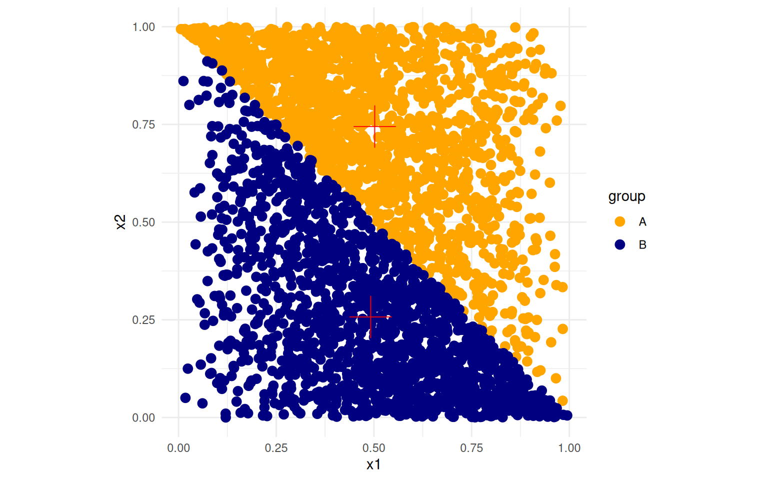

LDA model:

lda1 <- lda(group ~ x1 + x2, data = data, method = "moment")
data$lda <- predict(lda1)$class
data$class <- paste(data$group, data$lda)
ggplot(data, aes(x = x1, y = x2, colour = class, shape = group)) + geom_point(size = 3) +
    theme_minimal() + scale_color_manual(values = c("darkgreen", "orange", "red",
    "blue")) + geom_point(data = summ, aes(x = mx1, y = mx2), size = 10, shape = 3,
    color = "red") + coord_fixed()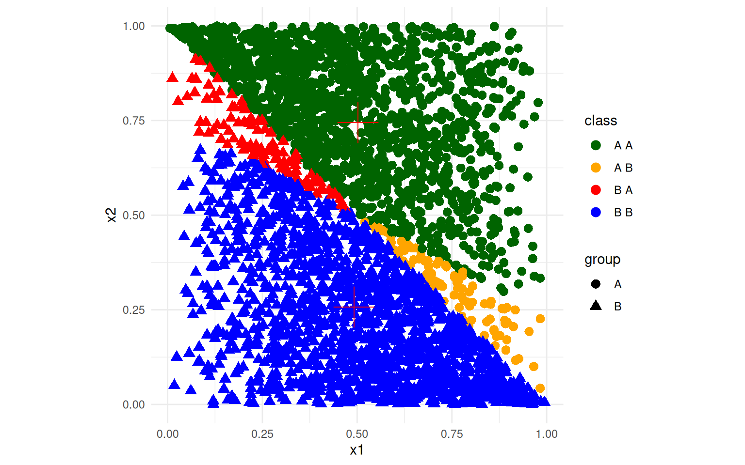

Here, although the classes are mostly correctly identified, the mapping onto the discriminant function means that the best line separating the two classes is not optimal–the angle is wrong.

SVM model:

svm1 <- svm(as.factor(group) ~ x1 + x2, data = data, kernel = "linear", scale = T)
data$svm <- predict(svm1)
data$classSVM <- paste(data$group, data$svm)
ggplot(data, aes(x = x1, y = x2, colour = classSVM, shape = group)) + geom_point(size = 3) +
    theme_minimal() + scale_color_manual(values = c("darkgreen", "orange", "red",
    "blue")) + coord_fixed()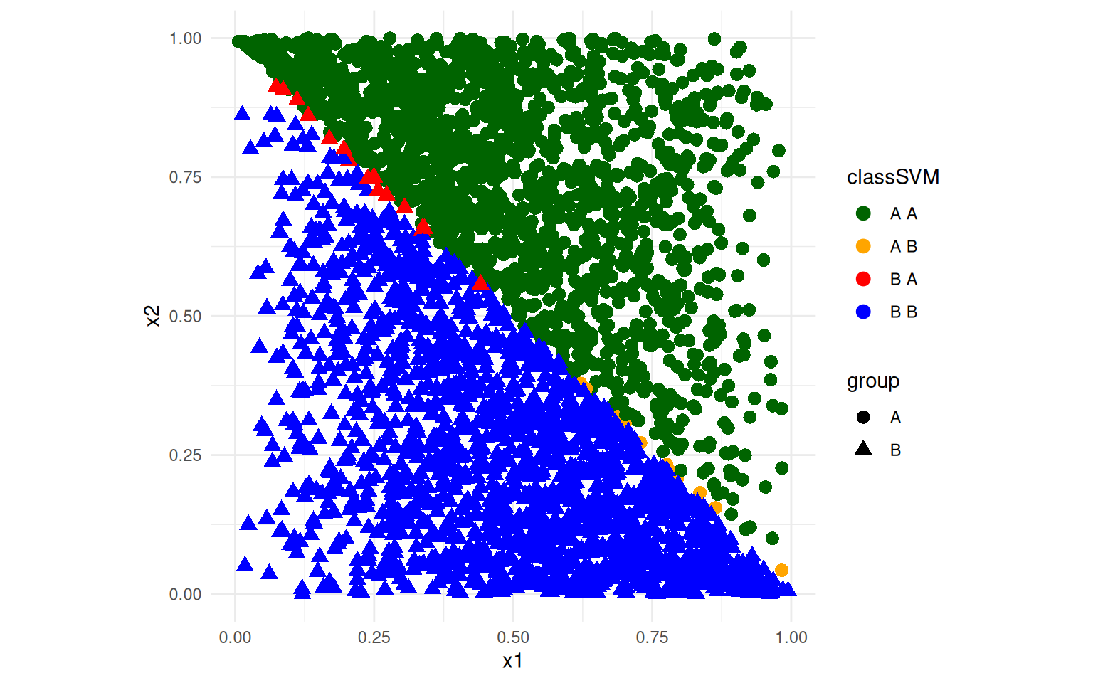

The SVM does a better job of separating the two groups. The LDA model is a linear model, but even though the groups are linearly seperable, the mapping onto the discriminant function means that the best line separating the two classes is not optimal. SVM uses optimization to find the best line based on the lines on the frontier between the two classes, and because it has more flexibility in the decision boundary, it can do a better job. T

A real data set

Let’s look at the engineering data set next. We will run a classifier on the engineering data first. Because the predicted variable is numeric, we will make it a factor so the svm knows to predict the class. The svm function needs to be told to use a linear svm, which seems reasonable in this case.

joint <- read.csv("eng-joint.csv")[, -1]
joint$eng <- as.factor(joint$eng)
s1 <- svm(y = joint$eng, x = joint[, -1], scale = T, kernel = "linear", cross = 5)

coef(s1)

(Intercept)         eer         eeu          ep         ppr         ppu 
 0.05154417 -0.15567504  0.16576103  0.36205481  0.25004473  0.57847773 
      eer.1       eeu.1        ep.1       ppr.1       ppu.1 
 0.10664820 -0.31357906  0.60989730 -0.43790979  0.40541747

summary(s1)


Call:
svm.default(x = joint[, -1], y = joint$eng, scale = T, kernel = "linear", 
    cross = 5)


Parameters:
   SVM-Type:  C-classification 
 SVM-Kernel:  linear 
       cost:  1 

Number of Support Vectors:  67

 ( 33 34 )


Number of Classes:  2 

Levels: 
 0 1

5-fold cross-validation on training data:

Total Accuracy: 40.78947 
Single Accuracies:
 60 40 26.66667 33.33333 43.75

confusion(joint$eng, predict(s1, data = joint))

Overall accuracy = 0.697 

Confusion matrix 
      Predicted (cv)
Actual     0     1
     0 0.684 0.316
     1 0.289 0.711

First, consider the arguments we gave. We specified that the variables should be rescaled–this makes sense here because the variables are on substantially different scales. Next, the svm used C-classification. This is the default for predicting factor values–if you give a numeric value to predict, it will implement a regression. You can also specify nu-classification which is essentially the same but uses a different parameter. Next, we used a linear kernel Different types of data (networks, sparse text-document matrices, images, etc.) are usually best fit by one or another of the available kernels. Next, the model specifies its ‘support vectors’. This is in a sense a number of parameters used to make the decisions. For linear classifiers, we can extract the coefficients–the actual plane used to discriminate between

The kernel trick for non-linear classifiers

If you cannot separate cleanly with a linear classifier, svm allows use of kernels (called the kernel trick). A kernel is just a way of transforming the features into a higher-dimensional space. Different kernels provide different higher-dimensional spaces, but essentially you can create new dimensions by combining existing features, enabling interactions and other complex classification patterns. A linear boundary on those new dimensions may produce a better classification. So the same SVM algorithm can apply after we generate a higher-dimensional representation. So rather than, for example, trying to find a curve that separates two classes of data, you transform the data into a higher-dimensional space that curves the data, and fit a linear separation in that space.

Polynomial kernel

A polynomial kernel provides something like polynomial regression. It might be worthwhile to examine a polynomial kernel, which is akin to QDA. We can see the fit improves to 79%

s1.pol <- svm(y = joint$eng, x = joint[, -1], kernel = "polynomial", scale = T)
s1.pol


Call:
svm.default(x = joint[, -1], y = joint$eng, scale = T, kernel = "polynomial")


Parameters:
   SVM-Type:  C-classification 
 SVM-Kernel:  polynomial 
       cost:  1 
     degree:  3 
     coef.0:  0 

Number of Support Vectors:  74

confusion(joint$eng, (predict(s1.pol)))

Overall accuracy = 0.789 

Confusion matrix 
      Predicted (cv)
Actual     0     1
     0 1.000 0.000
     1 0.421 0.579

The linear SVM does not do as well, while the polynomial performs better. But it gets 100% accuracy on the 0-0 cases, and does much more poorly on the 1-1 case. But these are as good or better than any of the other methods. The C-classification has two parameters that control the solution, the cost (C) of mis-classification and \(\gamma\). By increasing the cost function, we can punish errors more and force the model to fit the data better:

s1.pol <- svm(y = joint$eng, x = joint[, -1], kernel = "polynomial", scale = T, cost = 100)
s1.pol


Call:
svm.default(x = joint[, -1], y = joint$eng, scale = T, kernel = "polynomial", 
    cost = 100)


Parameters:
   SVM-Type:  C-classification 
 SVM-Kernel:  polynomial 
       cost:  100 
     degree:  3 
     coef.0:  0 

Number of Support Vectors:  60

confusion(joint$eng, (predict(s1.pol)))

Overall accuracy = 1 

Confusion matrix 
      Predicted (cv)
Actual 0 1
     0 1 0
     1 0 1

Cross-validation

The high error cost is likely leading to overfitting. It is also typical to use cross-validation to help determine reasonable values for the decision bounds. This svm library will do n-fold crossvalidation by specifying a cross argument Maybe that will help with overfitting.

s1.pol <- svm(y = joint$eng, x = joint[, -1], kernel = "polynomial", scale = T, cross = 10,
    cost = 100)
s1.pol$tot.accuracy

[1] 50

confusion(joint$eng, (predict(s1.pol)))

Overall accuracy = 1 

Confusion matrix 
      Predicted (cv)
Actual 0 1
     0 1 0
     1 0 1

It does not. This may in part be a limitation of the data, and probably of the polynomial kernel. But maybe the polynomial kernel is actually fairly good and not overfitting because it is finding areas of combined features that are especially diagnostic. To be sure, we might want to do our own held-out data set and see.

keep <- c(rep(T, 50), rep(F, 26))[order(runif(76))]
joint2 <- joint[keep, ]
s1.pol <- svm(y = joint2$eng, x = joint2[, -1], kernel = "polynomial", scale = T,
    cross = 10, cost = 100)
s1.pol$tot.accuracy

[1] 52

confusion(joint2$eng, (predict(s1.pol)))

Overall accuracy = 1 

Confusion matrix 
      Predicted (cv)
Actual 0 1
     0 1 0
     1 0 1

confusion(joint[!keep, ]$eng, (predict(s1.pol, newdata = joint[!keep, -1])))

Overall accuracy = 0.385 

Confusion matrix 
      Predicted (cv)
Actual     0     1
     0 0.375 0.625
     1 0.600 0.400

the held-out data is never fit very well.

RBF and sigmoid kernels

The radial basis function kernel is useful for especially for images, as it is sort of a guassian transformation of each pair of features. Similarly, a sigmoid kernel enables features to be combined using a similar combination, but it matches the sigmoid function used in neural networks. Let’s try the default kernel (radial) on the iphone data:

Exercise: iPhone data

phone <- read.csv("data_study1.csv")
phone$Smartphone <- factor(phone$Smartphone)
phone$Gender <- as.numeric(as.factor(phone$Gender))
phone.svm <- svm(y = phone$Smartphone, x = phone[, -1], scale = T, cross = 50)
phone.svm


Call:
svm.default(x = phone[, -1], y = phone$Smartphone, scale = T, cross = 50)


Parameters:
   SVM-Type:  C-classification 
 SVM-Kernel:  radial 
       cost:  1 

Number of Support Vectors:  429

summary(phone.svm)


Call:
svm.default(x = phone[, -1], y = phone$Smartphone, scale = T, cross = 50)


Parameters:
   SVM-Type:  C-classification 
 SVM-Kernel:  radial 
       cost:  1 

Number of Support Vectors:  429

 ( 227 202 )


Number of Classes:  2 

Levels: 
 Android iPhone

50-fold cross-validation on training data:

Total Accuracy: 63.32703 
Single Accuracies:
 70 72.72727 20 45.45455 70 54.54545 63.63636 60 63.63636 80 90.90909 80 45.45455 63.63636 80 63.63636 60 63.63636 54.54545 70 63.63636 50 36.36364 60 63.63636 72.72727 60 63.63636 60 54.54545 60 63.63636 63.63636 60 45.45455 60 63.63636 63.63636 50 81.81818 70 72.72727 80 63.63636 81.81818 60 81.81818 60 63.63636 63.63636

Here, we are about as good as other methods using cross-validation. It again would be worthwhile to select the C and gamma parameters via a grid search.

Exercise: MNist data

SVMs and the RBF kernel are especially well-suited for image data. We can use the image data, but this svm does not like features that have 0 variance, so let’s remove them.

train <- (read.csv("trainmnist.csv"))
var <- apply(train, 2, sd)
train2 <- train[, var > 0]
test <- as.matrix(read.csv("testmnist.csv")[, var > 0])
class <- as.factor(rep(c("0", "1"), each = 250))
mn.svm <- svm(y = class, x = train2, kernel = "radial", scale = F, cross = 10)
table(class, predict(mn.svm, test))

     
class   0   1
    0 249   1
    1   2 248

A trickier example

This example comes from Andrew Ng’s open classroom tutorials on SVMs (http://openclassroom.stanford.edu/MainFolder/DocumentPage.php?course=MachineLearning&doc=exercises/ex8/ex8.html)

ex4 <- read.csv("ex8a.csv", header = F)
ex4$V1 <- as.factor(ex4$V1)
ggplot(ex4, aes(x = V2, y = V3, colour = V1)) + geom_point(size = 3) + theme_minimal() +
    scale_color_manual(values = c("orange", "navy"))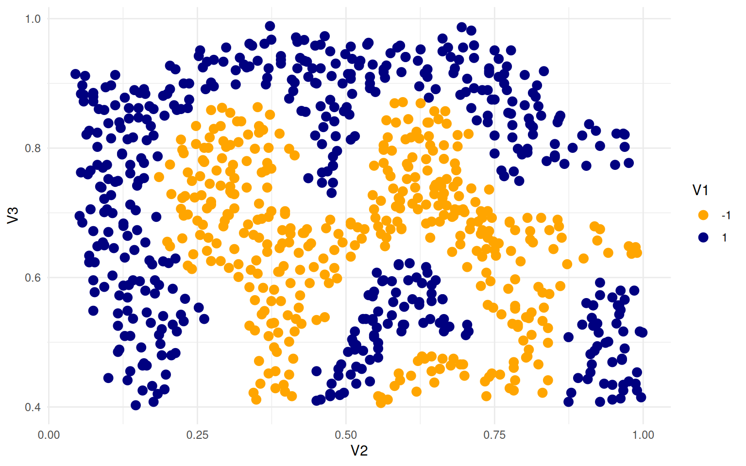

Here, we can try to create a SVM that separates the two sets, using a linear kernel:

# set.seed(100)
seed <- 20
set.seed(seed)
svm.ng <- svm(V1 ~ ., data = ex4[, 1:3], kernel = "linear", scale = F, cross = 10,
    cost = 10, fitted = T)
svm.ng


Call:
svm(formula = V1 ~ ., data = ex4[, 1:3], kernel = "linear", cross = 10, 
    cost = 10, fitted = T, scale = F)


Parameters:
   SVM-Type:  C-classification 
 SVM-Kernel:  linear 
       cost:  10 

Number of Support Vectors:  743

confusion(ex4$V1, predict(svm.ng))

Overall accuracy = 0.569 

Confusion matrix 
      Predicted (cv)
Actual    -1     1
    -1 0.462 0.538
    1  0.346 0.654

ex4$class <- predict(svm.ng)
ex4$class2 <- paste(ex4$V1, ex4$class)
ggplot(ex4, aes(x = V2, y = V3, colour = class2, shape = class)) + geom_point(size = 3) +
    theme_minimal() + scale_color_manual(values = c("darkgreen", "orange", "red",
    "blue"))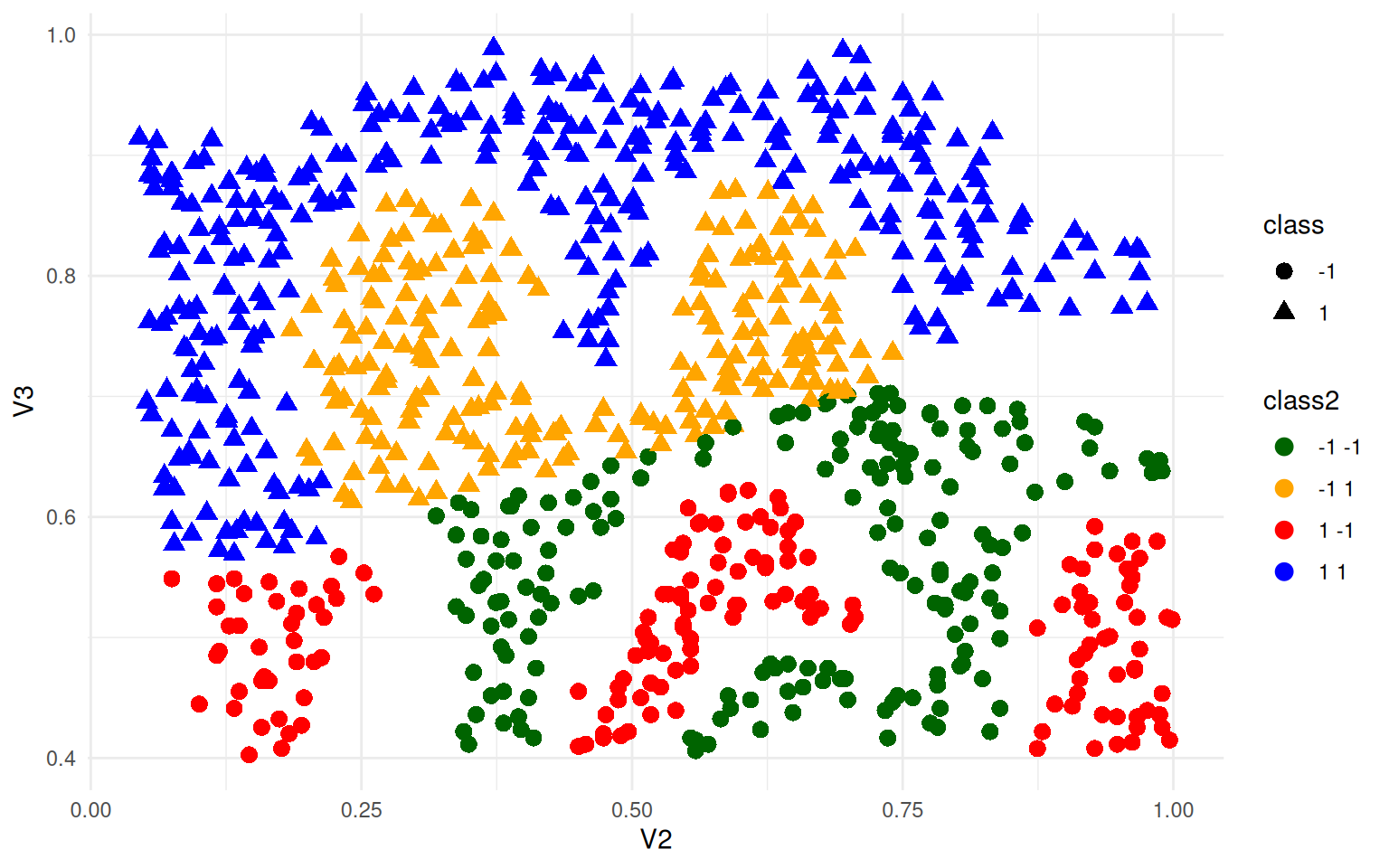

This used a linear kernel, and you can see it sort of splits the space in half and does horribly. The linear coefficients can be extracted:

coef(svm.ng)

(Intercept)          V2          V3 
 -2.0357351  -0.9325268   3.8319148

These coefficients specify a plane in v2/v3 that separates the two groups.

Let’s try again using a radial kernel:

svm.ng <- svm(V1 ~ ., data = ex4[, 1:3], kernel = "radial", scale = F, cross = 10,
    cost = 100, fitted = T)
svm.ng


Call:
svm(formula = V1 ~ ., data = ex4[, 1:3], kernel = "radial", cross = 10, 
    cost = 100, fitted = T, scale = F)


Parameters:
   SVM-Type:  C-classification 
 SVM-Kernel:  radial 
       cost:  100 

Number of Support Vectors:  439

confusion(ex4$V1, predict(svm.ng))

Overall accuracy = 0.824 

Confusion matrix 
      Predicted (cv)
Actual    -1     1
    -1 0.875 0.125
    1  0.217 0.783

ex4$class <- predict(svm.ng)
ex4$class2 <- paste(ex4$V1, ex4$class)
ggplot(ex4, aes(x = V2, y = V3, colour = class2, shape = class)) + geom_point(size = 3) +
    theme_minimal() + scale_color_manual(values = c("darkgreen", "orange", "red",
    "blue"))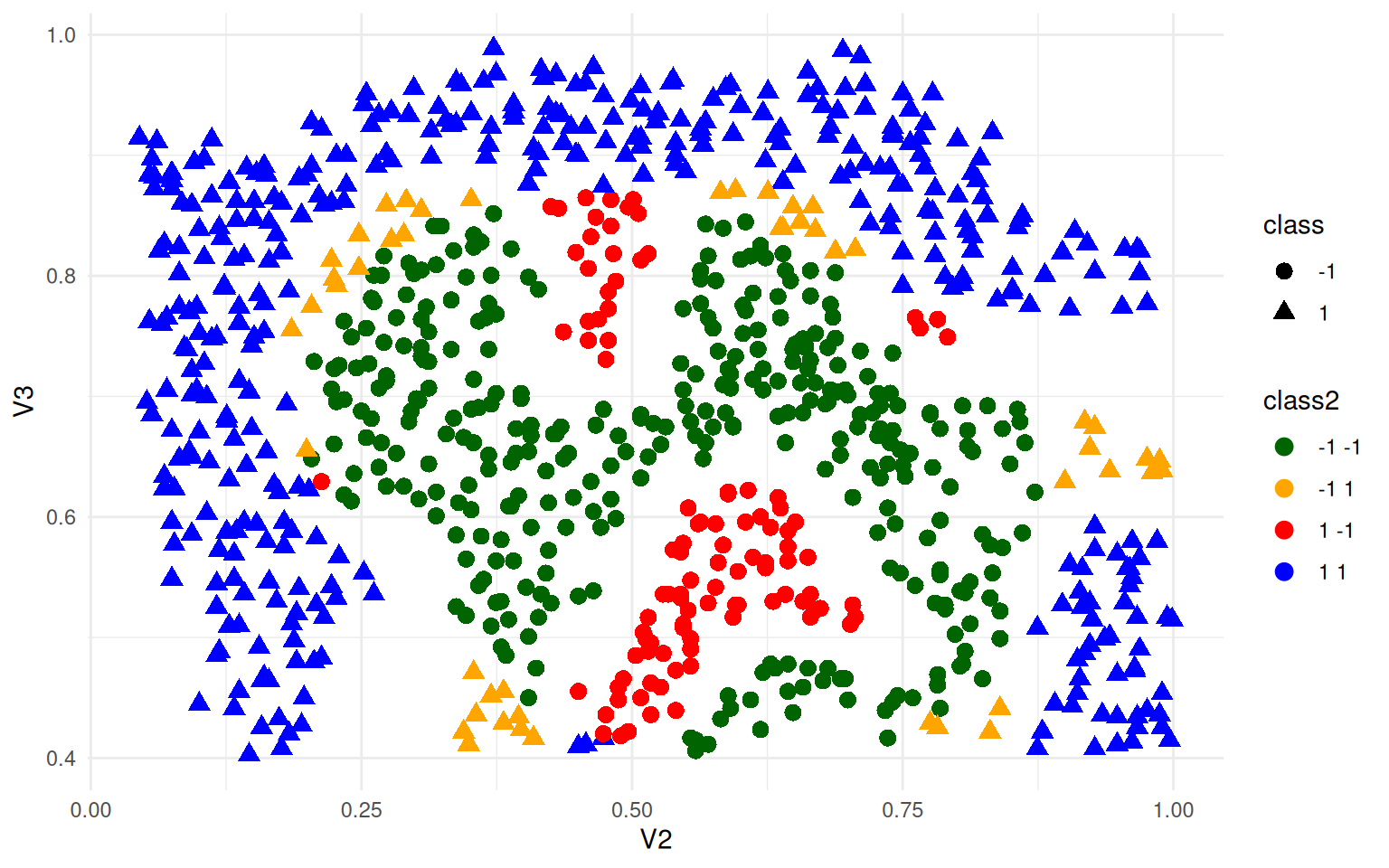

Here, green and blue are correct, and red/orange are incorrect. It creates a reasonably circle in the middle. Can we get better? The SVM is controlled by a parameter gamma, which is a sort of curvature parameter. Let’s try a large value of 100 (as suggested by Ng).

svm.ng <- svm(V1 ~ ., data = ex4[, 1:3], type = "nu-classification", kernel = "radial",
    scale = F, fitted = T, gamma = 100)
svm.ng


Call:
svm(formula = V1 ~ ., data = ex4[, 1:3], type = "nu-classification", 
    kernel = "radial", fitted = T, gamma = 100, scale = F)


Parameters:
   SVM-Type:  nu-classification 
 SVM-Kernel:  radial 
      gamma:  100 
         nu:  0.5 

Number of Support Vectors:  450

confusion(ex4$V1, predict(svm.ng))

Overall accuracy = 0.977 

Confusion matrix 
      Predicted (cv)
Actual    -1     1
    -1 0.958 0.042
    1  0.008 0.992

ex4$class <- predict(svm.ng)
ex4$class2 <- paste(ex4$V1, ex4$class)
ggplot(ex4, aes(x = V2, y = V3, colour = class2, shape = class)) + geom_point(size = 3) +
    theme_minimal() + scale_color_manual(values = c("darkgreen", "orange", "red",
    "blue"))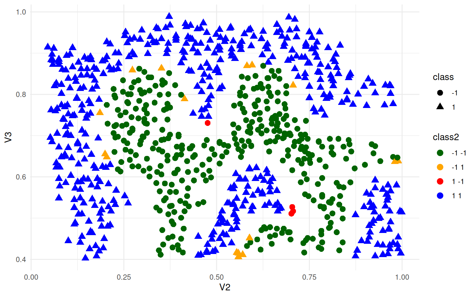

What if we added some noise and re-trained on data for which there was not as clear a boundary?

ex4b <- ex4
ex4b$V2 <- ex4b$V2 + rnorm(nrow(ex4), mean = 0, sd = 0.05)
ex4b$V3 <- ex4b$V3 + rnorm(nrow(ex4), mean = 0, sd = 0.05)

svm.ng <- svm(V1 ~ ., data = ex4b[, 1:3], kernel = "radial", scale = T, cross = 100,
    gamma = 100, cost = 0.5)
svm.ng


Call:
svm(formula = V1 ~ ., data = ex4b[, 1:3], kernel = "radial", cross = 100, 
    gamma = 100, cost = 0.5, scale = T)


Parameters:
   SVM-Type:  C-classification 
 SVM-Kernel:  radial 
       cost:  0.5 

Number of Support Vectors:  791

table(ex4b$V1, predict(svm.ng))

ex4b$class <- predict(svm.ng)
ex4b$class2 <- paste(ex4b$V1, ex4b$class)
ggplot(ex4b, aes(x = V2, y = V3, colour = class2, shape = class)) + geom_point(size = 3) +
    theme_minimal() + scale_color_manual(values = c("darkgreen", "orange", "red",
    "blue"))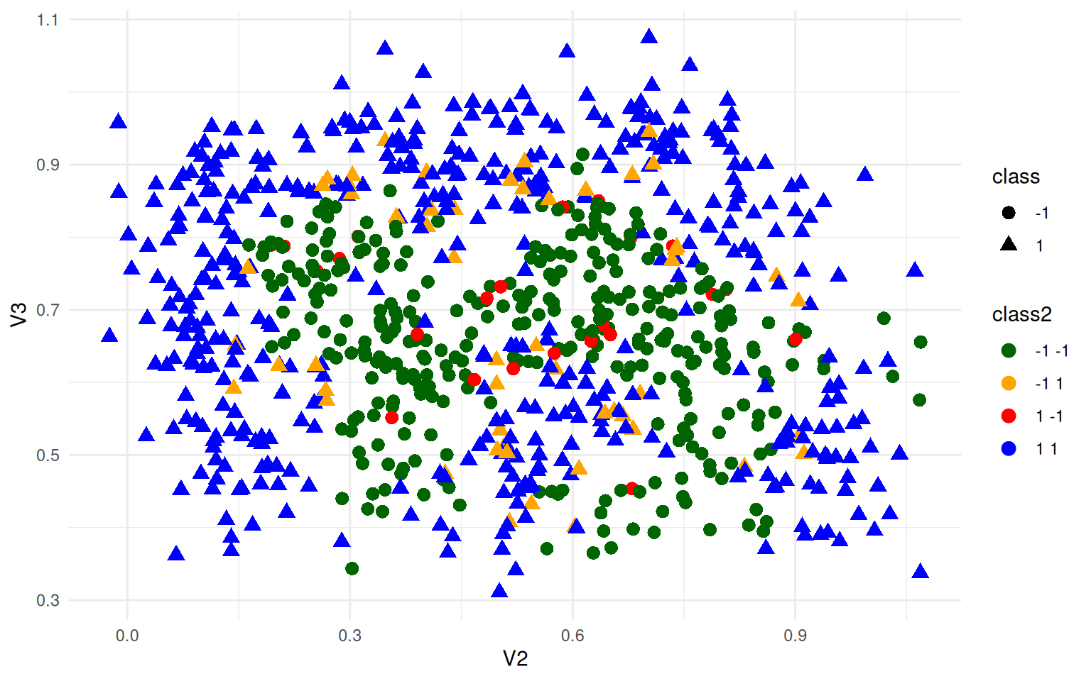

We can still do very well, just not 100% accuracy.

Summary

SVMs have a couple other functions, including regression and novelty detection. At their heart, they are quite similar to LDA, but use alternative methods for finding the best decision bound, and permit using kernels that generate new features (just like polynomial regression) enabling quite complicated non-linear classifiers.

Support Vector Machines