Simple Neural Network Classifiers

Artificial Neural Networks have been used by researchers since at least the 1950s, and rose in prominence when computing resources became widely available. There have been at least 3-4 eras of ANN, with each success and exuberance followed by a quiescence and failure or replacement by other tools. There has always been an intetrplay in this area between computational neuroscientists, computational vision, machine learning, psychology, computer science, and statisticians, with many advances coming by modeling human processes and then applying these algorithms to real-life problems.

In the 1950s, notions of the ANN were introduced (Perceptron, McCollough & Pitts)
In the 1960s, inadequacy of these methods were found (XOR problems), and
In the 1970s and 1980s, back-propagation provided a reasonable learning approach for multi-layer neural networks for supervised classification problems (Rumelhart & McClelland).
In the 1970s-1990s, other advances in self-organizing maps, un-supervised learning and hebbian networks provided alternate means for representing knowledge.
In the 1990s-2000s, other machine learning approaches appeared to take precedence, with lines blurring between ANNs, machine classification, reinforcement learning, and several approaches that linked supervised and unsupervised models (O’Reilly, HTMs, Grossberg).
In the 2000s, Bayesian approaches were foremost
In the 2010s, we have seen a resurgence of deep-learning methods. The advances here have been driven by (1) advances in software that allow us to use GPU (graphics cards) to efficiently train and use networks (2) large data labeled data sets, often generated through amazon mechanical turk or as a byproduct of CAPTCHA systems; (3) using 15+ hidden layers; (4) effective use of specific types of layer architectures, including convolutional networks that de-localize patterns from their position in an image.

A simple two-layer neural network can be considered that is essentially what our multinomial regression or logistic regression model is doing. Inputs include a set of features, and output nodes (possibly one per class) are classifications that are learned. Alterately, a pattern can be learned by the output nodes. The main issue here is estimating weights, which are done with heuristic error-propagation approaches rather than MLE or least squares. This is inefficient for two-layer problems, but the heuristic approach will pay off for more complex problems.

The main advance of the late 1970s and early 1980s was adoption of ‘hidden layer’ ANNs. These hidden layers permit solving the XOR problem: when a class is associated with an exclusive or logic. The category structure is stored in a distributed fashion across all nodes, but there is a sense in which the number of hidden nodes controls how complex the classification structure that is possible. With a hidden layer, optimization is difficult with traditional means, but the heuristic approaches generally work reasonably well.

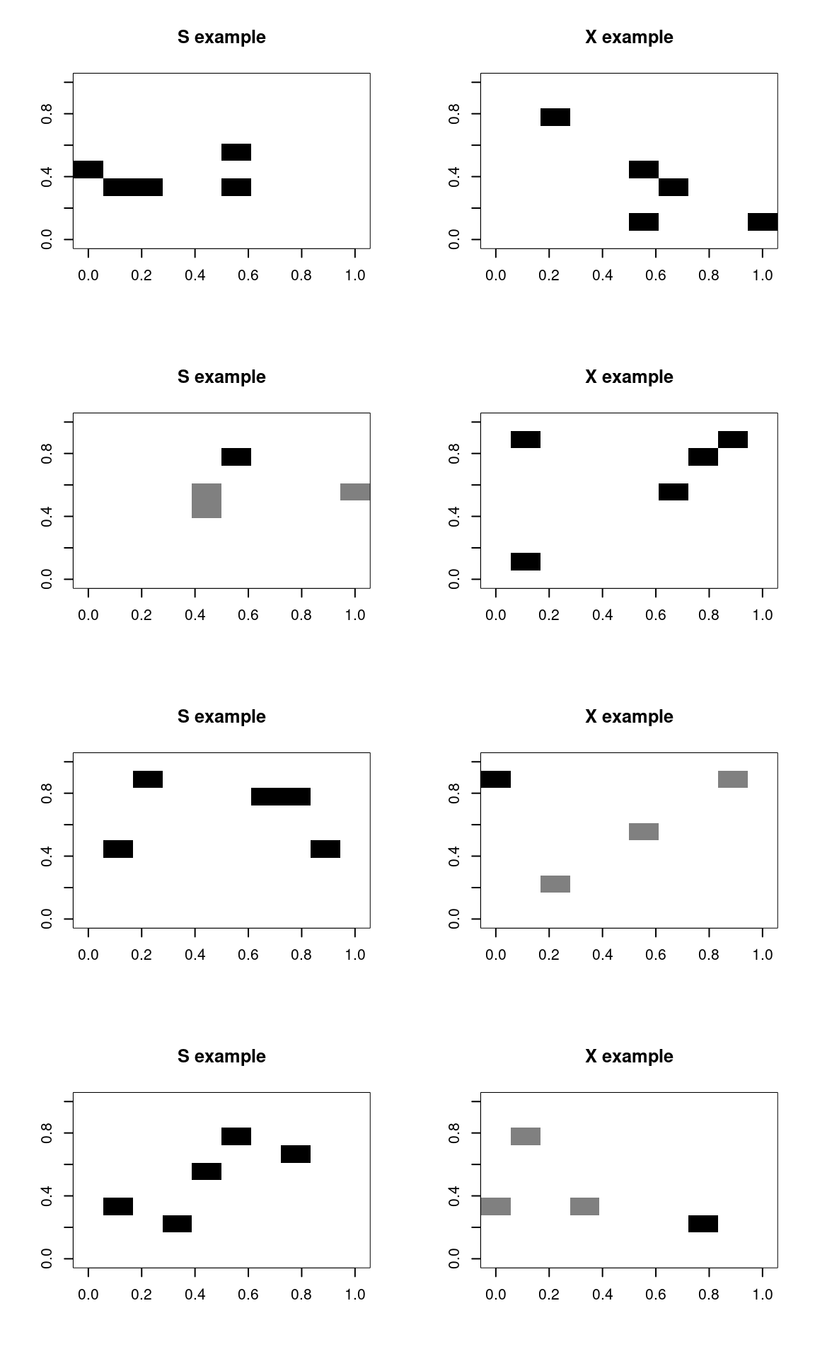
We will start with an image processing example. We will take two images (S and X) and sample features from them to make exemplars:

# library(imager) s <-load.image('s.data.bmp') x <- load.image('x.bmp') svec <-
# as.vector(s) xvec <- as.vector(x) write.csv(svec,'s.csv')
# write.csv(xvec,'x.csv')

## here, the lower the value, the darker the image.
svec <- read.csv("s.csv")
xvec <- read.csv("x.csv")

## reverse the numbers
svec$x <- 255 - svec$x
xvec$x <- 255 - xvec$x

par(mfrow = c(1, 2))

image(matrix(svec$x, 10, 10, byrow = T), col = grey(100:0/100))
image(matrix(xvec$x, 10, 10, byrow = T), col = grey(100:0/100))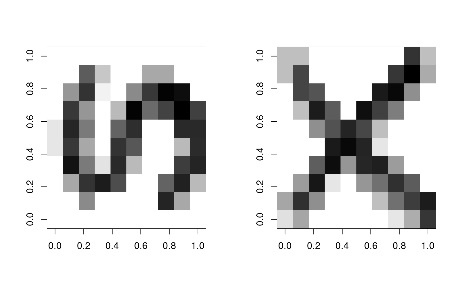

To train the model, we will sample 500 examples of each template:

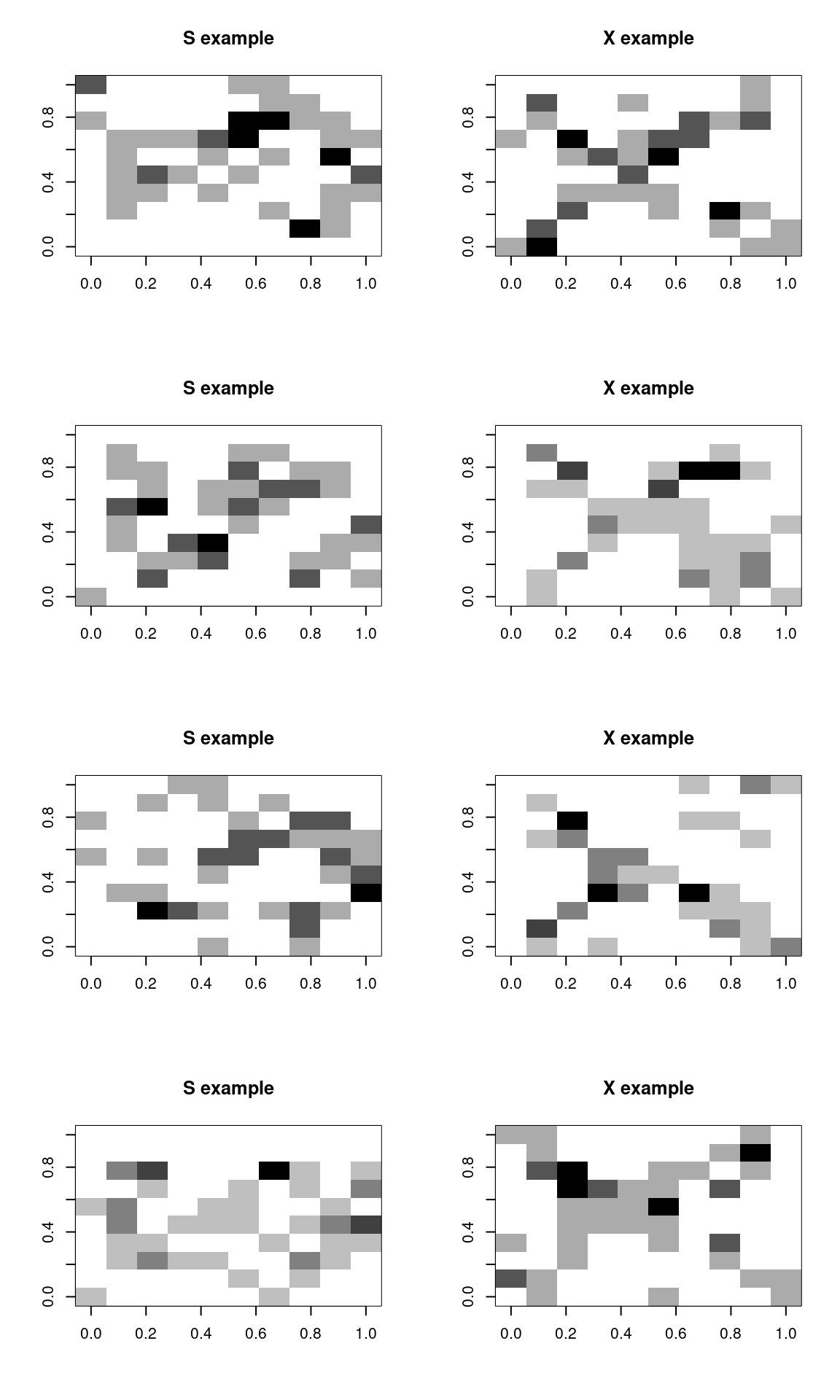
dataX <- matrix(0, ncol = 100, nrow = 250)
dataS <- matrix(0, ncol = 100, nrow = 250)
letter <- rep(c("x", "s"), each = 250)

par(mfrow = c(4, 2))

for (i in 1:250) {
    x <- rep(0, 100)
    xtmp <- table(sample(1:100, size = 50, prob = as.matrix(xvec$x), replace = T))
    x[as.numeric(names(xtmp))] <- xtmp/max(xtmp)

    s <- rep(0, 100)
    stmp <- table(sample(1:100, size = 50, prob = as.matrix(svec$x), replace = T))
    s[as.numeric(names(stmp))] <- stmp/max(stmp)

    if (i <= 4) {
        image(matrix(s, 10, 10, byrow = T), main = "S example", col = grey(100:0/100))
        image(matrix(x, 10, 10, byrow = T), main = "X example", col = grey(100:0/100))
    }

    dataX[i, ] <- x
    dataS[i, ] <- s
}

data <- rbind(dataX, dataS)

Let’s train a neural network on these. Note that we could probably have trained it on the prototypes–maybe from the mnist library examined in earlier chapters.

library(nnet)
options(warn = 2)
# model <- nnet(letter~data,size=2) #This doesn't work.

# Let's transform the letter to a numeric value
model <- nnet(y = as.numeric(letter == "s"), x = data, size = 2)

# weights:  205
initial  value 134.702308 
final  value 0.000000 
converged

model

a 100-2-1 network with 205 weights
options were -

# alternately, try using letter as a factor, and use a formula. This also plays
# with some of the learning parameters
merged <- data.frame(letter = as.factor(letter), data)
model2 <- nnet(letter ~ ., data = merged, size = 2, rang = 0.1, decay = 1e-04, maxit = 500,
    trace = T)

# weights:  205
initial  value 346.322926 
iter  10 value 0.978601
iter  20 value 0.059554
iter  30 value 0.045672
iter  40 value 0.044185
iter  50 value 0.043833
iter  60 value 0.043422
iter  70 value 0.043135
iter  80 value 0.042890
iter  90 value 0.042723
iter 100 value 0.042618
iter 110 value 0.042548
iter 120 value 0.042533
iter 130 value 0.042527
iter 140 value 0.042525
iter 150 value 0.042525
iter 150 value 0.042525
iter 150 value 0.042525
final  value 0.042525 
converged

Examining the model

The model contains a lot of information, including some parameters it is constructed under, and all of the fitted parameters.
We can see when using summary() that we really have two really large regressions from the 100 input features to 2 hidden nodes, and a single model with an intercept (b=bias) and two parameters from each hidden node to the output node. The default is ‘logistic output units’, which means this last model is essentially a logistic regression.

str(model)

List of 15
 $ n            : num [1:3] 100 2 1
 $ nunits       : int 104
 $ nconn        : num [1:105] 0 0 0 0 0 0 0 0 0 0 ...
 $ conn         : num [1:205] 0 1 2 3 4 5 6 7 8 9 ...
 $ nsunits      : int 104
 $ decay        : num 0
 $ entropy      : logi FALSE
 $ softmax      : logi FALSE
 $ censored     : logi FALSE
 $ value        : num 0
 $ wts          : num [1:205] 6.514 16.642 54.629 -2.507 -0.751 ...
 $ convergence  : int 0
 $ fitted.values: num [1:500, 1] 0 0 0 0 0 0 0 0 0 0 ...
  ..- attr(*, "dimnames")=List of 2
  .. ..$ : NULL
  .. ..$ : NULL
 $ residuals    : num [1:500, 1] 0 0 0 0 0 0 0 0 0 0 ...
  ..- attr(*, "dimnames")=List of 2
  .. ..$ : NULL
  .. ..$ : NULL
 $ call         : language nnet.default(x = data, y = as.numeric(letter == "s"), size = 2)
 - attr(*, "class")= chr "nnet"

summary(model)

a 100-2-1 network with 205 weights
options were -
  b->h1  i1->h1  i2->h1  i3->h1  i4->h1  i5->h1  i6->h1  i7->h1  i8->h1  i9->h1 
   6.51   16.64   54.63   -2.51   -0.75  -11.67  -19.44    0.27   -4.66   34.21 
i10->h1 i11->h1 i12->h1 i13->h1 i14->h1 i15->h1 i16->h1 i17->h1 i18->h1 i19->h1 
  22.85   42.93  103.99   14.77 -136.22 -106.21 -104.15  -62.49   37.18   96.57 
i20->h1 i21->h1 i22->h1 i23->h1 i24->h1 i25->h1 i26->h1 i27->h1 i28->h1 i29->h1 
  34.94   -1.57    3.97   20.70   24.06  -44.29   -5.45   58.42  -14.75  -95.98 
i30->h1 i31->h1 i32->h1 i33->h1 i34->h1 i35->h1 i36->h1 i37->h1 i38->h1 i39->h1 
  -0.71   -4.40    1.53 -107.80   93.82  114.35   87.75   81.22   -7.13  -32.74 
i40->h1 i41->h1 i42->h1 i43->h1 i44->h1 i45->h1 i46->h1 i47->h1 i48->h1 i49->h1 
 -10.22   -5.16    2.86  -95.27  -59.75   38.84   19.13  -33.20    1.48    1.50 
i50->h1 i51->h1 i52->h1 i53->h1 i54->h1 i55->h1 i56->h1 i57->h1 i58->h1 i59->h1 
   0.89   -3.79   -1.54   59.90   74.24   18.12  -10.47   -5.23  -53.03   -3.33 
i60->h1 i61->h1 i62->h1 i63->h1 i64->h1 i65->h1 i66->h1 i67->h1 i68->h1 i69->h1 
  -0.20   -3.76   30.26   70.65  114.12    9.66   28.29   11.55    9.78  -50.00 
i70->h1 i71->h1 i72->h1 i73->h1 i74->h1 
  -9.48   11.66  -29.55   30.64   50.13 
 [ reached getOption("max.print") -- omitted 26 entries ]
  b->h2  i1->h2  i2->h2  i3->h2  i4->h2  i5->h2  i6->h2  i7->h2  i8->h2  i9->h2 
  55.36   11.09   39.59   -1.45    0.80   -4.54  -10.06    2.82   -2.64   26.02 
i10->h2 i11->h2 i12->h2 i13->h2 i14->h2 i15->h2 i16->h2 i17->h2 i18->h2 i19->h2 
  19.54   34.08   79.86   14.69  -80.55  -60.74  -58.17  -32.11   35.50   69.24 
i20->h2 i21->h2 i22->h2 i23->h2 i24->h2 i25->h2 i26->h2 i27->h2 i28->h2 i29->h2 
  28.54    0.02   10.45   24.45   24.28  -23.31    6.52   50.81    7.18  -54.88 
i30->h2 i31->h2 i32->h2 i33->h2 i34->h2 i35->h2 i36->h2 i37->h2 i38->h2 i39->h2 
   0.20   -0.41    3.07  -56.86   69.01   83.03   63.17   58.35   -1.15  -17.86 
i40->h2 i41->h2 i42->h2 i43->h2 i44->h2 i45->h2 i46->h2 i47->h2 i48->h2 i49->h2 
  -4.14   -0.41    3.49  -53.29  -28.35   41.55   27.99  -18.03    2.85    1.25 
i50->h2 i51->h2 i52->h2 i53->h2 i54->h2 i55->h2 i56->h2 i57->h2 i58->h2 i59->h2 
   1.96   -0.50    0.02   41.41   57.65   23.97    7.79   14.33  -31.03    0.58 
i60->h2 i61->h2 i62->h2 i63->h2 i64->h2 i65->h2 i66->h2 i67->h2 i68->h2 i69->h2 
   0.83    1.60   23.59   52.50   79.37    9.06   23.07   18.62   20.15  -28.00 
i70->h2 i71->h2 i72->h2 i73->h2 i74->h2 
  -4.23    9.64   -4.37   33.46   37.92 
 [ reached getOption("max.print") -- omitted 26 entries ]
   b->o   h1->o   h2->o 
  57.16 -460.68  363.91

Some of the arguments we can control are:

How the final output classifier works (options involve linout, entropy, softmax, censored). These control fitting algorithms and approaches, and may impact speed of convergence. The default settings look like they are essentially using least-squared to fit individual nodes.
subset: allowing you to train on a subset for cross-validation
mask: allowing only some of the input features to be trained.
Wts: initial parameter settings. You could train a model on some data, and use those weights to then re-train on new data, for example.
decay: this probably controls how far back data in a series are examined. It may allow for a model to adapt to a changing environment better.
maxit and trace: fitting arguments.
weights: strength of each case. You may have some cases you want to train on more strongly/often.

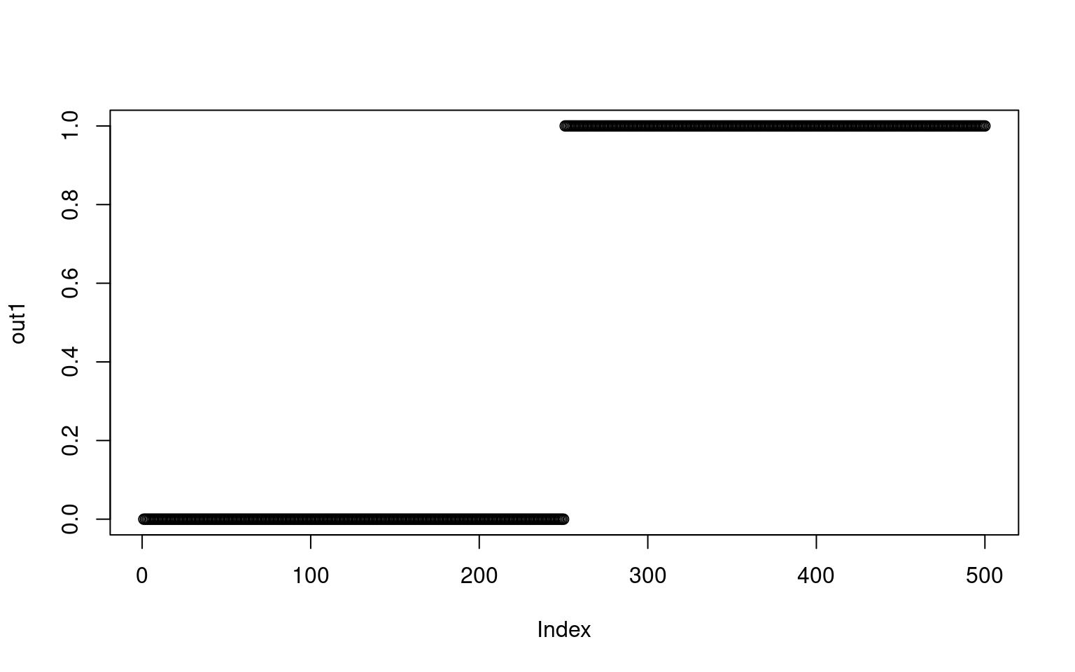
Obtaining predicted response

When we use predict, by default it gives us the ‘raw’ values–activation values returned by the trained network. Because the final layer of this network has just one node (100-2-1), it is just an activation value indicating the class (0 for X and 1 for S). The values are not exactly 0 and 1–they are floating point values very close.

out1 <- predict(model, newdata = data)
plot(out1)

If there were a combined example that was hard to distinguish we would get a different value:

test <- (data[3, ] + data[255, ])/2

par(mfrow = c(1, 3))
image(matrix(data[3, ], 10), col = grey(100:0/100))
image(matrix(data[255, ], 10), col = grey(100:0/100))
image(matrix(test, 10), col = grey(100:0/100))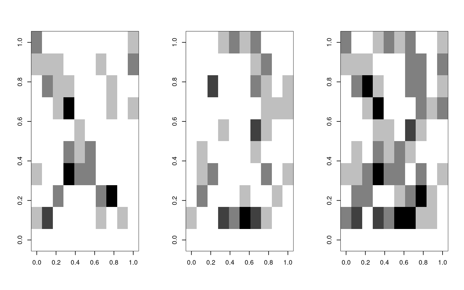

predict(model, newdata = data[3, ] + data[4, ])

     [,1]
[1,]    0

predict(model, newdata = data[255, ])

     [,1]
[1,]    1

predict(model, newdata = test)

     [,1]
[1,]    1

In this case, the X shows up as a strong X, the S shows up as an S, but the combined version is a slightly weaker S.

We can get classifications using type=“class”:

predict(model2, type = "class")

 [1] "x" "x" "x" "x" "x" "x" "x" "x" "x" "x" "x" "x" "x" "x" "x" "x" "x" "x" "x"
[20] "x" "x" "x" "x" "x" "x" "x" "x" "x" "x" "x" "x" "x" "x" "x" "x" "x" "x" "x"
[39] "x" "x" "x" "x" "x" "x" "x" "x" "x" "x" "x" "x" "x" "x" "x" "x" "x" "x" "x"
[58] "x" "x" "x" "x" "x" "x" "x" "x" "x" "x" "x" "x" "x" "x" "x" "x" "x" "x"
 [ reached getOption("max.print") -- omitted 425 entries ]

table(letter, predict(model2, type = "class"))

      
letter   s   x
     s 250   0
     x   0 250

Training with very limited/noisy examples

This classification is actually perfect, but there was a lot of information available. Let’s sample just 5 points out to create the pattern:

dataX <- matrix(0, ncol = 100, nrow = 250)
dataS <- matrix(0, ncol = 100, nrow = 250)
letter <- rep(c("x", "s"), each = 250)


par(mfrow = c(4, 2))

for (i in 1:250) {
    x <- rep(0, 100)
    xtmp <- table(sample(1:100, size = 5, prob = as.matrix(xvec$x), replace = T))
    x[as.numeric(names(xtmp))] <- xtmp/max(xtmp)

    s <- rep(0, 100)
    stmp <- table(sample(1:100, size = 5, prob = as.matrix(svec$x), replace = T))
    s[as.numeric(names(stmp))] <- stmp/max(stmp)

    ## plot the first few examples:
    if (i <= 4) {
        image(matrix(s, 10, 10, byrow = T), main = "S example", col = grey(100:0/100))
        image(matrix(x, 10, 10, byrow = T), main = "X example", col = grey(100:0/100))
    }
    dataX[i, ] <- x
    dataS[i, ] <- s
}

data <- rbind(dataX, dataS)



merged <- data.frame(letter = as.factor(letter), data)
model3 <- nnet(letter ~ ., data = merged, size = 2, rarg = 0.1, decay = 1e-04, maxit = 500)

# weights:  205
initial  value 349.342458 
iter  10 value 98.547003
iter  20 value 45.166893
iter  30 value 30.523416
iter  40 value 28.985007
iter  50 value 28.355796
iter  60 value 27.688482
iter  70 value 26.956694
iter  80 value 26.550998
iter  90 value 24.582976
iter 100 value 24.418685
iter 110 value 24.330491
iter 120 value 24.206411
iter 130 value 23.996977
iter 140 value 23.323214
iter 150 value 19.973030
iter 160 value 16.959922
iter 170 value 14.900277
iter 180 value 14.703310
iter 190 value 14.631866
iter 200 value 14.591938
iter 210 value 14.543914
iter 220 value 14.432881
iter 230 value 14.355548
iter 240 value 14.329130
iter 250 value 14.301357
iter 260 value 14.187941
iter 270 value 14.062408
iter 280 value 14.031454
iter 290 value 14.021345
iter 300 value 14.014148
iter 310 value 14.007568
iter 320 value 14.000887
iter 330 value 13.931244
iter 340 value 13.867128
iter 350 value 13.827783
iter 360 value 7.780889
iter 370 value 7.504392
iter 380 value 7.436209
iter 390 value 7.396963
iter 400 value 7.350464
iter 410 value 7.309284
iter 420 value 7.276907
iter 430 value 7.246058
iter 440 value 7.222203
iter 450 value 7.201361
iter 460 value 7.191541
iter 470 value 7.185425
iter 480 value 7.178740
iter 490 value 7.172972
iter 500 value 7.162451
final  value 7.162451 
stopped after 500 iterations

table(letter, predict(model3, type = "class"))

      
letter   s   x
     s 250   0
     x   1 249

It still does very well, with a few errors, for very sparse data. In fact, it might be doing TOO well. That is, in a sense, it is picking up on arbitrary but highly diagnostic features. A human observer would never be confident in the outcome, because the information is too sparse, but in this limited world, a single pixel is enough to make a good guess.

Neural Networks and the XOR problem

Neural networks became popular when researchers realized that networks with a hidden layer could solve ‘XOR classification problems’. Early on, researchers recognized that a simple perception (2-layer) neural network could be used for AND or OR combinations, but not XOR, as these are not linearly separable. XOR classification maps onto many real-world interaction problems. For example, two safe pharmaceuticals might be dangerous when taken together, and a simple neural network could never detect this state–if one is good, and the other is good, both must be better. An XOR problem is one in which one feature or another (but not both or neither) indicate class membership. In order to perform classification with this logic, a hidden layer is required.

Here is a class defined by an XOR structure:

library(MASS)
library(DAAG)
feature1 <- rnorm(200)
feature2 <- rnorm(200)
outcome <- as.factor((feature1 > 0.6 & feature2 > 0.3) | (feature1 > 0.6 & feature2 <
    0.3))
outcome <- as.factor((feature1 * (-feature2) + rnorm(200)) > 0)

The linear discriminant model fails to discriminate (at least without an interaction)

lmodel <- lda(outcome ~ feature1 + feature2)

confusion(outcome, predict(lmodel)$class)

Overall accuracy = 0.6 

Confusion matrix 
       Predicted (cv)
Actual  FALSE  TRUE
  FALSE 0.387 0.613
  TRUE  0.215 0.785

lmodel2 <- lda(outcome ~ feature1 * feature2)

confusion(outcome, predict(lmodel2)$class)

Overall accuracy = 0.695 

Confusion matrix 
       Predicted (cv)
Actual  FALSE  TRUE
  FALSE 0.602 0.398
  TRUE  0.224 0.776

Similarly, the neural networks with an empty single layer (skip=TRUE) are not great at discriminating, but with a few hidden nodes they work well.

n1 <- nnet(outcome ~ feature1 + feature2, size = 0, skip = TRUE)

# weights:  3
initial  value 153.137485 
final  value 136.081429 
converged

confusion(outcome, factor(predict(n1, type = "class"), levels = c(TRUE, FALSE)))

Overall accuracy = 0.4 

Confusion matrix 
       Predicted (cv)
Actual  FALSE  TRUE
  FALSE 0.613 0.387
  TRUE  0.785 0.215

n2 <- nnet(outcome ~ feature1 + feature2, size = 3, skip = TRUE)

# weights:  15
initial  value 149.958156 
iter  10 value 107.371535
iter  20 value 105.720295
iter  30 value 104.412357
iter  40 value 104.161983
iter  50 value 104.043551
iter  60 value 103.894953
iter  70 value 103.831541
iter  80 value 103.562693
iter  90 value 103.424503
iter 100 value 103.399276
final  value 103.399276 
stopped after 100 iterations

confusion(outcome, factor(predict(n2, type = "class"), levels = c(FALSE, TRUE)))

Overall accuracy = 0.695 

Confusion matrix 
       Predicted (cv)
Actual  FALSE  TRUE
  FALSE 0.774 0.226
  TRUE  0.374 0.626

Because we have the XOR structure, the simple neural network without a hidden layer is essentially LDA, and in fact often gets a similar level of accuracy (53%).

IPhone Data using the NNet

To model the iphone data set, we need to decide on how large of a model we want. We need to also remember that training a model like this is not deterministic–every time we do it the situation will be a little different. Because we have just two classes, maybe a 2-layer hidden network would work.

By fitting the model several times, we can see that it performs differently every time. At times, the model does reasonably well. This does about as well as any of the best classification models. Curiously, this particular model has a bias toward Android accuracy.

phone <- read.csv("data_study1.csv")
phone$Smartphone <- (as.factor(phone$Smartphone))
phone$Gender <- as.numeric(as.factor(phone$Gender))
set.seed(100)
phonemodel <- nnet(Smartphone ~ ., size = 3, data = phone)

# weights:  43
initial  value 368.669183 
iter  10 value 351.629336
iter  20 value 328.109320
iter  30 value 319.345472
iter  40 value 317.075499
iter  50 value 314.039955
iter  60 value 313.953479
final  value 313.953382 
converged

confusion(phone$Smartphone, factor(predict(phonemodel, newdata = phone, type = "class",
    levels = c("Android", "iPhone"))))

Overall accuracy = 0.652 

Confusion matrix 
         Predicted (cv)
Actual    Android iPhone
  Android   0.603  0.397
  iPhone    0.313  0.687

Other times, it does poorly: Here, it calls everything an iPhone:

set.seed(101)
phonemodel2 <- nnet(Smartphone ~ ., data = phone, size = 2)

# weights:  29
initial  value 457.289985 
final  value 358.808683 
converged

confusion(phone$Smartphone, factor(predict(phonemodel2, newdata = phone, type = "class"),
    levels = c("Android", "iPhone")))

Overall accuracy = 0.586 

Confusion matrix 
         Predicted (cv)
Actual    Android iPhone
  Android       0      1
  iPhone        0      1

In this case, it called everything in iPhone, resulting in 58.6% accuracy. Like many of our approaches, we are doing heuristic optimization and so may end up in local optima. It is thus useful to run the model many several times and look for the best model. Running this many times, the best models seem to get around 370-390 correct, which is in the low 70% for accuracy.

preds <- matrix(0, 100)
for (i in 1:100) {
    phonemodel3 <- nnet(Smartphone ~ ., data = phone, size = 2)
    preds[i] <- confusion(phone$Smartphone, factor(predict(phonemodel3, newdata = phone,
        type = "class"), levels = c("Android", "iPhone")))$overall

}

hist(preds, col = "gold", main = "Accuracy of 100 fitted models (2 hidden nodes)",
    xlim = c(0, 1))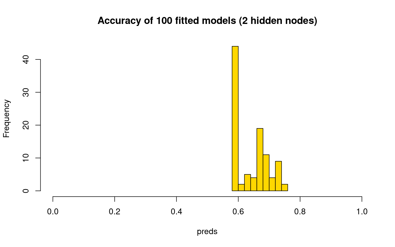

Do we do any better, on average, with more hidden nodes?

preds <- matrix(0, 100)
for (i in 1:100) {
    phonemodel3 <- nnet(Smartphone ~ ., data = phone, size = 6)
    preds[i] <- confusion(phone$Smartphone, factor(predict(phonemodel3, newdata = phone,
        type = "class"), levels = c("Android", "iPhone")))$overall

}

hist(preds, col = "gold", main = "Accuracy of 100 fitted models (6 hidden nodes)",
    xlim = c(0, 1))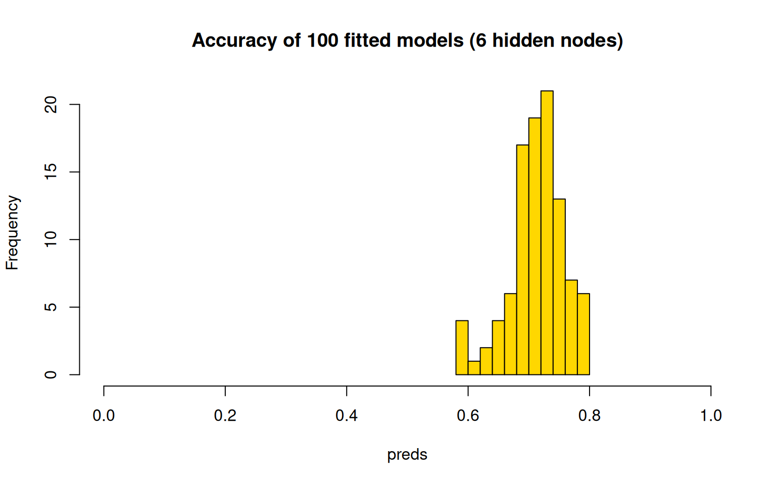

This seems to be more consistent, and do better overall–usually above 70% accuracy. But like every model we have examined, the best models are likely to be over-fitting, and getting lucky at re-predicting their own data. It would also be important to implement a cross-validation scheme. There is no built-in cross-validation here, but you can implement one using subset functions.

train <- rep(FALSE, nrow(phone))
train[sample(1:nrow(phone), size = 300)] <- TRUE
test <- !train

phonemodel2 <- nnet(Smartphone ~ ., data = phone, size = 6, subset = train)

# weights:  85
initial  value 204.327276 
iter  10 value 193.352724
iter  20 value 166.957659
iter  30 value 136.845896
iter  40 value 126.652225
iter  50 value 118.844038
iter  60 value 114.601579
iter  70 value 112.362718
iter  80 value 109.187074
iter  90 value 106.922061
iter 100 value 104.486444
final  value 104.486444 
stopped after 100 iterations

confusion(phone$Smartphone[test], predict(phonemodel2, newdata = phone[test, ], type = "class"))

Overall accuracy = 0.563 

Confusion matrix 
         Predicted (cv)
Actual    Android iPhone
  Android   0.340  0.660
  iPhone    0.273  0.727

We can try this 100 times and see how well it does on the cross-validation set:

preds <- rep(0, 100)

for (i in 1:100) {
    train <- rep(FALSE, nrow(phone))
    train[sample(1:nrow(phone), size = 300)] <- TRUE
    test <- !train

    phonemodel2 <- nnet(Smartphone ~ ., data = phone, size = 6, subset = train)
    preds[i] <- confusion(phone$Smartphone[test], factor(predict(phonemodel2, newdata = phone[test,
        ], type = "class"), levels = c("Android", "iPhone")))$overall

}

hist(preds, col = "gold", main = "Accuracy of 100 cross-validated models (6 hidden nodes)",
    xlim = c(0, 1))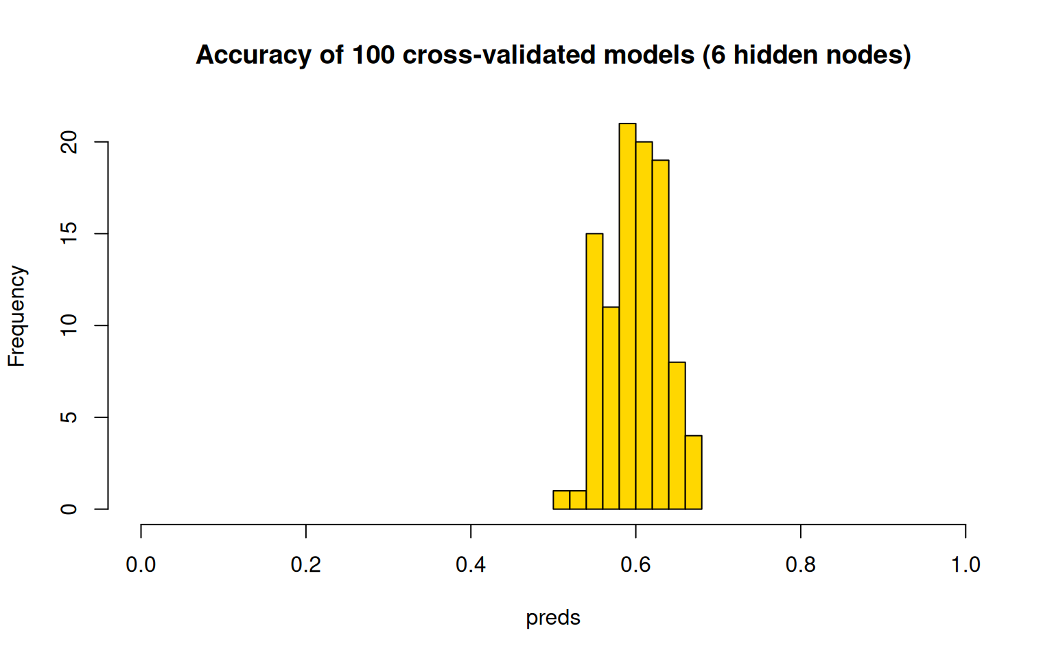

The cross-validation scores are typically a bit lower, with models getting around 60% on average, and up to 70% for the best. Now that we have built this, we could use average cross-validation accuracy to help select variables for exclusion. Here, let’s just test the predictors we have found previously to be fairly good:

preds <- rep(0, 100)

for (i in 1:100) {
    train <- rep(FALSE, nrow(phone))
    train[sample(1:nrow(phone), size = 300)] <- TRUE
    test <- !train

    phonemodel2 <- nnet(Smartphone ~ Gender + Avoidance.Similarity + Phone.as.status.object +
        Age, data = phone, size = 6, subset = train)
    preds[i] <- confusion(phone$Smartphone[test], factor(predict(phonemodel2, newdata = phone[test,
        ], type = "class"), levels = c("Android", "iPhone")))$overall

}

hist(preds, col = "gold", main = "Accuracy of 100 cross-validated models (6 hidden nodes)",
    xlim = c(0, 1))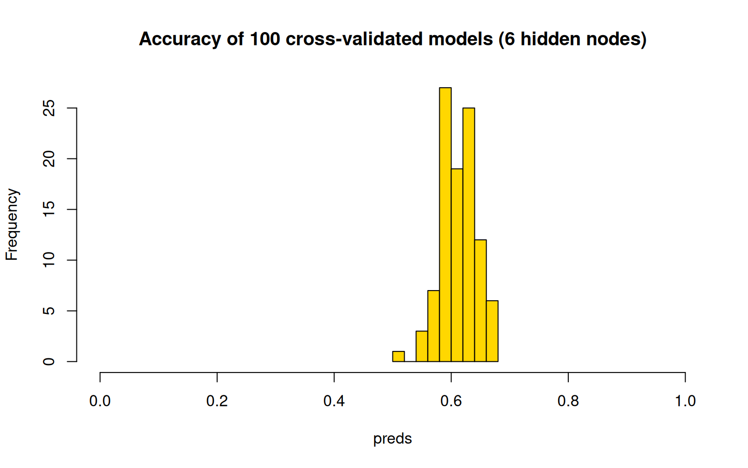

Most of these are better than chance, and it seems to do about as well as the full set of predictors as well.

The `neuralnet` library

The neuralnet library is perhaps a more flexible implementation, with multiple hidden layers. Here we have 2 hidden layers with two nodes each. When fitting it, it seemed to get stuck frequently and not converge or have some other error, but it does give a nice graphical visualization of the network. It seems to used more advanced backprop algorithms and activation functions. Here we have two hidden layers with two nodes each. The network does not make a lot of sense, but the model fails to converge under many larger network conditions.

library(neuralnet)
set.seed(10313)
train <- rep(FALSE, nrow(phone))
train[sample(1:nrow(phone), size = 300)] <- TRUE
test <- !train

phonemodel3 <- neuralnet(Smartphone ~ ., hidden = c(2, 2), data = phone[train, ])

pred <- apply(predict(phonemodel3, newdata = phone[test, ]), 1, which.max)
ptest <- phone[test, ]
acc <- (sum(ptest[pred == 1, ]$Smartphone == "Android") + sum(ptest[pred == 2, ]$Smartphone ==
    "iPhone"))/sum(test)
print(acc)

[1] 0.5764192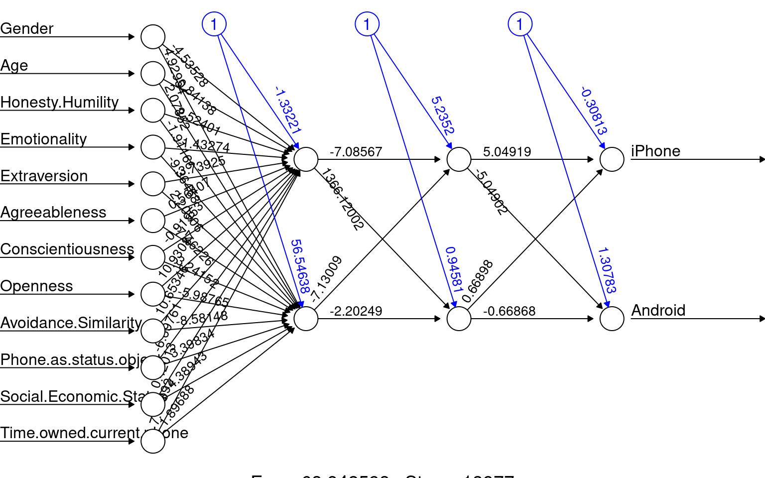

plot(phonemodel3, rep = "best")

Classifying handwritten characters using a neural net

The neuralnet library is a bit more powerful, and allows multiple layers. Let’s try it for a larger data set–mnist handwritten characters. I’ve included 10,000 cases inn mnist_test.csv, but this gets a bit difficult to build a model, so let’s consider three characters that are similar: 4, 7, and 9. This results in about 3000 cases, so lets fit the data on a subset of 1000, using 10 hidden nodes.

library(neuralnet)
library(DAAG)
## 10K examples of 0 to 9
mnistdat <- read.csv("mnist_test.csv")
mnistdat$label <- factor(mnistdat$label)  ## this needs to be a factor if it has more than 2 levels

mnist47 <- mnistdat[mnistdat$label == 4 | mnistdat$label == 7 | mnistdat$label ==
    9, ]

train <- mnist47[sample(1:nrow(mnist47), 1000), ]  #train on some examples
set.seed(100)
mnist <- neuralnet(label ~ ., hidden = c(4), data = train)

## examine the trained data:
table(train$label, c(4, 7, 9)[apply(mnist$response, 1, which.max)])

   
      4   7   9
  0   0   0   0
  1   0   0   0
  2   0   0   0
  3   0   0   0
  4 319   0   0
  5   0   0   0
  6   0   0   0
  7   0 358   0
  8   0   0   0
  9   0   0 323

p2 <- predict(mnist, newdata = mnist47)
pred <- c(4, 7, 9)[apply(p2, 1, which.max)]

table(mnist47$label, pred)

   pred
      4   7   9
  0   0   0   0
  1   0   0   0
  2   0   0   0
  3   0   0   0
  4 654  10 318
  5   0   0   0
  6   0   0   0
  7  17 906 105
  8   0   0   0
  9  72  36 901

mean(mnist47$label == pred)

[1] 0.8151706

Errors of 4 categorized as a 7:

error47 <- mnist47[mnist47$label == 4 & pred == 7, ]
cols <- grey(100:1/100)
par(mfrow = c(2, 4))
image((matrix(as.numeric(error47[1, -1]), nrow = 28, ncol = 28))[, 28:1], xaxt = "n",
    yaxt = "n", col = cols, main = "4s called 7s")
image((matrix(as.numeric(error47[2, -1]), nrow = 28, ncol = 28))[, 28:1], xaxt = "n",
    yaxt = "n", col = cols, main = "4s called 7s")
image((matrix(as.numeric(error47[3, -1]), nrow = 28, ncol = 28))[, 28:1], xaxt = "n",
    yaxt = "n", col = cols, main = "4s called 7s")
image((matrix(as.numeric(error47[4, -1]), nrow = 28, ncol = 28))[, 28:1], xaxt = "n",
    yaxt = "n", col = cols, main = "4s called 7s")
image((matrix(as.numeric(error47[5, -1]), nrow = 28, ncol = 28))[, 28:1], xaxt = "n",
    yaxt = "n", col = cols, main = "4s called 7s")
image((matrix(as.numeric(error47[6, -1]), nrow = 28, ncol = 28))[, 28:1], xaxt = "n",
    yaxt = "n", col = cols, main = "4s called 7s")
image((matrix(as.numeric(error47[7, -1]), nrow = 28, ncol = 28))[, 28:1], xaxt = "n",
    yaxt = "n", col = cols, main = "4s called 7s")
image((matrix(as.numeric(error47[8, -1]), nrow = 28, ncol = 28))[, 28:1], xaxt = "n",
    yaxt = "n", col = cols, main = "4s called 7s")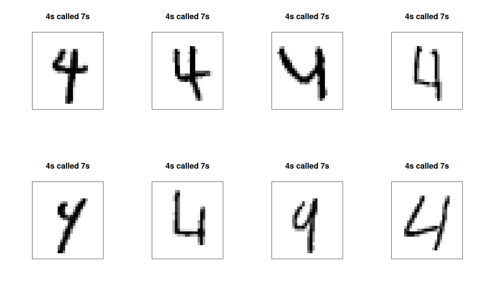

Errors of 4 categorized as a 9:

error49 <- mnist47[mnist47$label == 4 & pred == 9, ]
cols <- grey(100:1/100)
par(mfrow = c(2, 4))
image((matrix(as.numeric(error49[1, -1]), nrow = 28, ncol = 28))[, 28:1], xaxt = "n",
    yaxt = "n", col = cols, main = "4s called 7s")
image((matrix(as.numeric(error49[2, -1]), nrow = 28, ncol = 28))[, 28:1], xaxt = "n",
    yaxt = "n", col = cols, main = "4s called 7s")
image((matrix(as.numeric(error49[3, -1]), nrow = 28, ncol = 28))[, 28:1], xaxt = "n",
    yaxt = "n", col = cols, main = "4s called 7s")
image((matrix(as.numeric(error49[4, -1]), nrow = 28, ncol = 28))[, 28:1], xaxt = "n",
    yaxt = "n", col = cols, main = "4s called 7s")
image((matrix(as.numeric(error49[5, -1]), nrow = 28, ncol = 28))[, 28:1], xaxt = "n",
    yaxt = "n", col = cols, main = "4s called 7s")
image((matrix(as.numeric(error49[6, -1]), nrow = 28, ncol = 28))[, 28:1], xaxt = "n",
    yaxt = "n", col = cols, main = "4s called 7s")
image((matrix(as.numeric(error49[7, -1]), nrow = 28, ncol = 28))[, 28:1], xaxt = "n",
    yaxt = "n", col = cols, main = "4s called 7s")
image((matrix(as.numeric(error49[8, -1]), nrow = 28, ncol = 28))[, 28:1], xaxt = "n",
    yaxt = "n", col = cols, main = "4s called 7s")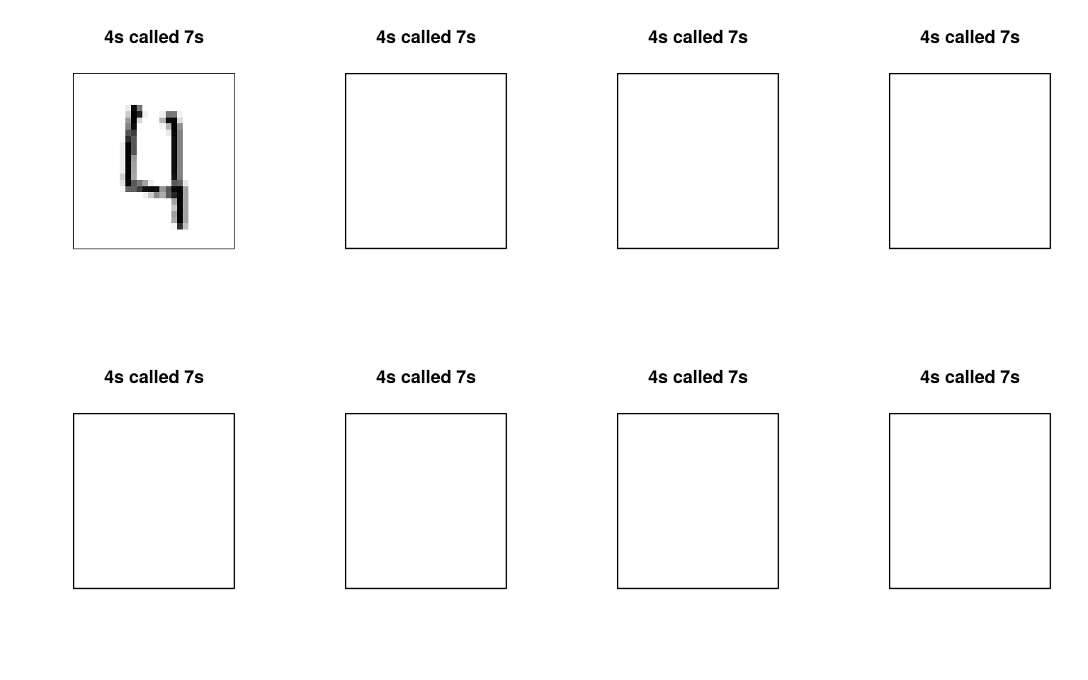

We can maybe see some patterns here for what kinds of errors are being made.

This is just the tip of the iceberg for neural network models. Modern deep networks use a mixture of different kinds of sublayers that are specialized for handling specific kinds of data (e.g., recurrent, convolutional, etc.), and they also use 15+ layers. These require substantial compute power to fit, and huge data sets of labeled data–often labeled by humans. But this is the basis for many of the recent advances in artificial intelligence.

Simple Neural Network Classifiers