Clustering Methods
Return to course site
Clustering Methods
Additional Reading: Venables & Ripley MASS Chapter 11
This unit covers a handful of clustering approaches, including k-means clustering, a number of hierarchical clustering approaches (divisive and agglomerative), and variations on these methods.
Clustering Approaches
Previously, we examined MDS, that attempted to find a coordinate system to map items into based on their (dis)similarity. Sometimes this revealed fuzzy groups, and other times just dimensions in space that were sometimes interpretable. During the unit on machine classification, we covered partitioning approaches that tried to find ways of grouping data together based on simple decision rules to best predict a specific category. What happens if you don’t know the identity, but still want to come up with bottom-up categories? We can use a distance metric to identify groups without knowing their labels–a general approach called clustering.
Just like MDS, clustering approaches find ways of grouping data together based on implied dissimilarity, which can sometimes be interpreted as ‘distance’. We assume that we have either measured or can compute a dissimilarity score (akin to a distance) for every pair of items. If we have this dissimilarity measure or can transform our measure to be a dissimilarity measure, these approaches are feasible. Interestingly, when we were covering MDS, we said that if you have a feature based representation, you might use PCA directly instead of transforming feature coding into a similarity space and then re-inducing a metric space from that similarity space. For most of the clustering methods we will consider in this unit, we similarly need a distance space, and end up computing one and throwing out the initial feature representation. This is not universally true for all clustering methods (e.g., finite mixture modeling does not do this), but it is an assumption clustering approaches make that inferred distance measures are an accurate depiction of the similarity space.
Psychological Distance
Many times, similarity ratings and behavioral measures (errors or response time) are treated as a indexing a psychological distance. However, this analogy is often mistaken and misleading, as argued by Tversky (1975). Most examples of subjective similarity (or dissimilarity) violate one or another of the axioms of metric spaces, which say that (1; identity) The distance between something and itself is 0; (2. symmetry) the distance between A and B is the same as the distance between B and A; and (3. triangle inequality) the D(A,B) + D(B,C)> D(A,C). This last one is hard to satisfy in subjective similarity: frosted flakes are similar to cheerios, and cheerios are similar to bagels, but frosted flakes are not similar to bagels. This means that for ratings such as this, distance is the wrong metaphor to use to understand what is going on, and maybe that scaling approaches (to be covered later) and factor analytic approaches are flawed as well, as they assume metric properties that might not exist.
Basic Approaches to clustering
If you have the goal of developing a clustering solution, there are two basic approaches (and hybrids between them). On one side, you could start with the notion of making a complete hierarchical description of all the elements. This is like a complete partitioning tree, where every element ends up being a leaf in the tree. The tree can then be examined for structure, or potentially chopped off to reveal the most important clusters. Everything is in multiple clusters of different levels. These methods are called ```hierarchical clustering’’’ methods. On the other hand, you might start with an assumption that there are a fixed number of groups. Based on that assumption, you may try to find the best arrangement of elements into clusters that fits your assumptions. This might be called a finite clustering method, and is typified by k-means clustering and related techniques. There are hybrids, especially within Bayesian approaches, that permit an infinite number of groups, and different optimization/inference approaches, including Bayesian inference and E-M optimization. The traditional approaches use distance measures directly, and include both agglomerative and divisive approaches to hierarchical clustering and k-means and related methods for finite clustering.
Hierarchical Clustering
Tversky made several suggestions to account for the findings, based primarily on the fact that different features are weighted differently. This seems to favor an approach where data can be partitioned based on dissimilarity of one feature, such that if two things differ on an important feature, matches along less important features might not matter. He suggested a hierarchical clustering approach to characterize data of this sort.
In a hierarchical approach, you create a binary tree, so that the first split divides the population into two groups that are most different, and each sub-population is split, recursively, until everything is on its own leaf. There are a number of ways to do this, but the final solution provides a complete set of dissimilarity measures that are ‘’ultra-metric’’ when visualized in a tree. The dissimilarity between any two elements is interpreted as the measure of the largest group that contains both items. Note that we throw away the complete dissimilarity matrix and replace it with one inferred by the cluster. Sometimes this works and we have a useful representation.
Sample Data: Alphabet Similarity
The example below uses the response time data to different letter pairs as an example.
distmat0 <- as.matrix(read.csv("plaindist.csv")[, -1])
colnames(distmat0) <- LETTERS
rownames(distmat0) <- LETTERS
distmat0[1:5, 1:5]
A B C D E
A 0.00000 61.10980 76.51373 61.25098 60.34510
B 61.10980 0.00000 50.77647 28.70588 23.72941
C 76.51373 50.77647 0.00000 46.55686 44.63922
D 61.25098 28.70588 46.55686 0.00000 34.51373
E 60.34510 23.72941 44.63922 34.51373 0.00000## Transform it into distance matrix
distmat <- as.dist(distmat0)
image(1:26, 1:26, distmat0, xaxt = "n", yaxt = "n", main = "Similarity of letters",
xlab = "", ylab = "")
axis(1, 1:26, LETTERS, cex.axis = 0.75)
axis(2, 1:26, LETTERS, cex.axis = 0.75)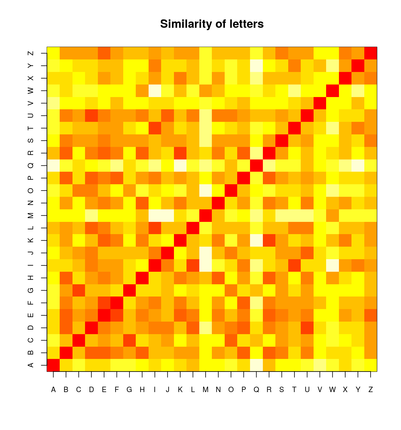
Along with the subjective similarity rating data, we can often give clustering algorithms feature or dimensional data. For comparison, we will look at a feature-level analysis of letters produced by Keren & Baggen (1981). Here, the features include things like roundness, horizontal, vertical features, and the like.
  V2 V3 V4 V5 V6 V7 V8 V9 V10 V11 V12 V13 V14 V15
A  0  0  1  1  1  0  0  1   0   0   0   1   0   0
B  1  1  0  1  1  0  0  0   1   0   1   0   0   0
C  1  0  0  0  0  0  0  0   1   0   1   0   0   1
D  1  1  0  0  0  0  0  0   1   0   1   0   0   0
E  1  0  0  1  0  0  0  0   0   0   1   0   0   1
 [ reached getOption("max.print") -- omitted 21 rows ]
Notice that distmat has been pre-processed and scaled to produce a distance-like measure. The diagonal is always 0, but what else shows up? It is hard to say for sure. We could apply and MDS like before to understand the space.
initial  value 27.327755
iter   5 value 20.670653
iter  10 value 18.888452
iter  15 value 18.107814
final  value 17.999589
converged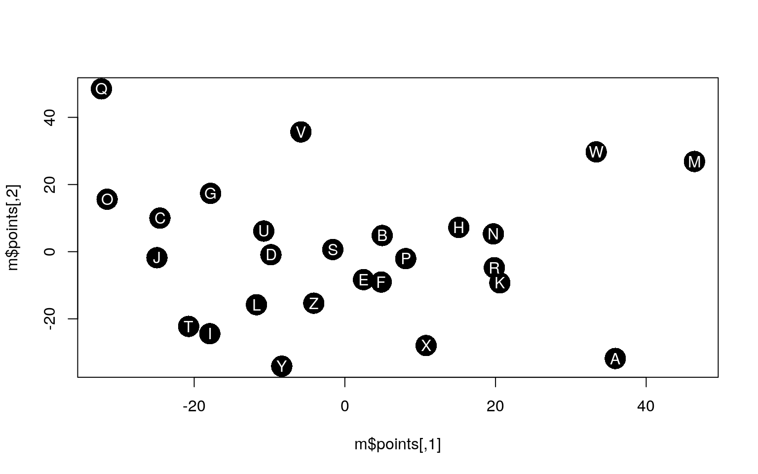 The MDS puts similarly-shaped letters in similar positions. However, a clustering approach may show other things. First, we will consider hierarchical clustering methods. Hierarchical clustering attempts to find a hierarchy that groups or divides items repeatedly until the whole set is characterized by a binary tree. In order to do this, we need to decide on whether we want to start from the bottom (called agglomerative), merging pairs together, then adding groups together, until the entire data set is merged, or start at the top (called divisive), repeatedly dividing sets in ways that maximize within-set similarity and minimize between-set similarity. Once we decide on the direction, we also needs to determine a method for defining what ‘close’ means when we want to divide or merge items and clusters. For example, do we count the similarity of two groups to be the largest of the inter-cluster similarity, the smallest, the average, or something else. We will start by examining the clustering methods in the \(cluster\) library.
The cluster library
Several clustering methods are available within the cluster library. A hierarchical clustering might look like this. We will start with agnes, an agglomerative clustering approach. This is bottom-up, and finds the closest pairs at each stage to link together, linking items and existing clusters together until the entire set is linked.
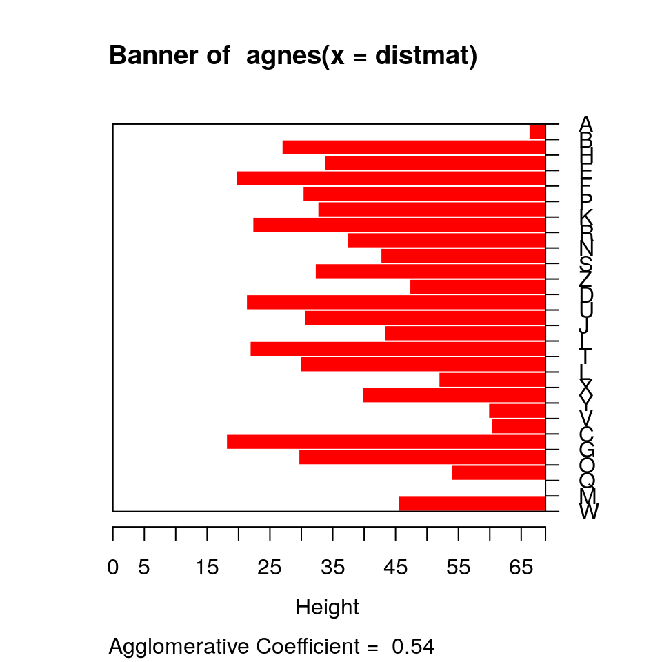
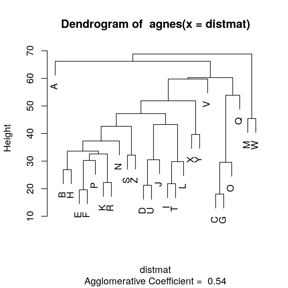
The standard display plot is sometimes not very polished. The ggdendro package provides a ggplot-based visualization:

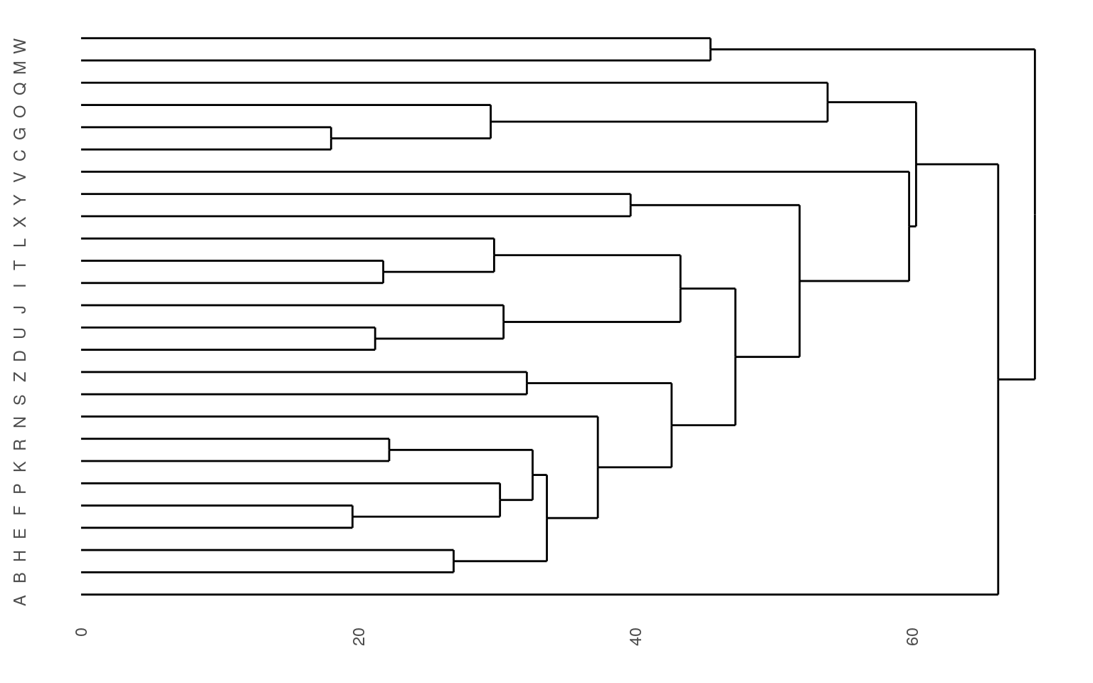
Notice that at the very bottom, we typically have visually-similar letters grouped. As you move higher, there are larger clusters that are more broadly similar. But dissimilarity is less clear. With appropriate distance measures, a hierarchical clustering is an ‘’ultrametric’’. Here, we interpret the dissimilarity between two things is the height of the cluster containing them both. Here, A, is dissimilar to everything; C, G, O, and Q are in a cluster, with Q being somewhat least well fit, and so on. Ultrametric spaces are convenient when the similarity between two things only matters locally, and if you get far away everything is essentially equally dissimilar.
The cluster library provides a set of functions for creating hierarchical and other clusters. They allows you to either specify the raw data or a distance metric. If you specify the raw data, it will compute a distance metric based on either euclidean or manhattan distance. Warning…if you give it a distance measure but don’t transform it into one using as.dist, it can still give you something that looks OK, but is wrong. Compare the following, using the ‘agnes’ function. Remember that distmat0 matrix, which was the original raw data; distmat is the one that had been turned into a distance object.
library(gridExtra)
library(ggplot2)
p1 <- ggdendrogram(agnes(distmat))
p2 <- ggdendrogram(agnes(distmat0))
grid.arrange(p1, p2)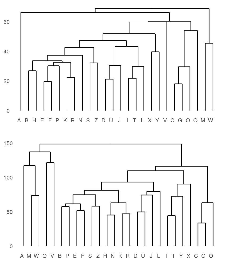 They both look sort of reasonable, but the first one is better. The second one is treating the distance matrix as if it were a set of features–it then creates a distance matrix based on these features, which ends up being fairly similar but not identical. In some cases, it could be very different, so you need to be careful about what goes into these functions.
If you specify a set of features, you also can specify the type of metric used to compute a distance. The two available are euclidean and manhattan. Euclidean distance is just distance in space as the crow flies. Manhattan distance takes the deviation along each dimension and sums them–it is distance as you would need to travel along a city block scheme. The second is often better if you have independent features that don’t trade off.
Agglomerative approaches
The agglomerative approach implemented within the agnes function starts by finding pairs that go together, and then build up from the bottom. Let’s look more carefully at what happens:
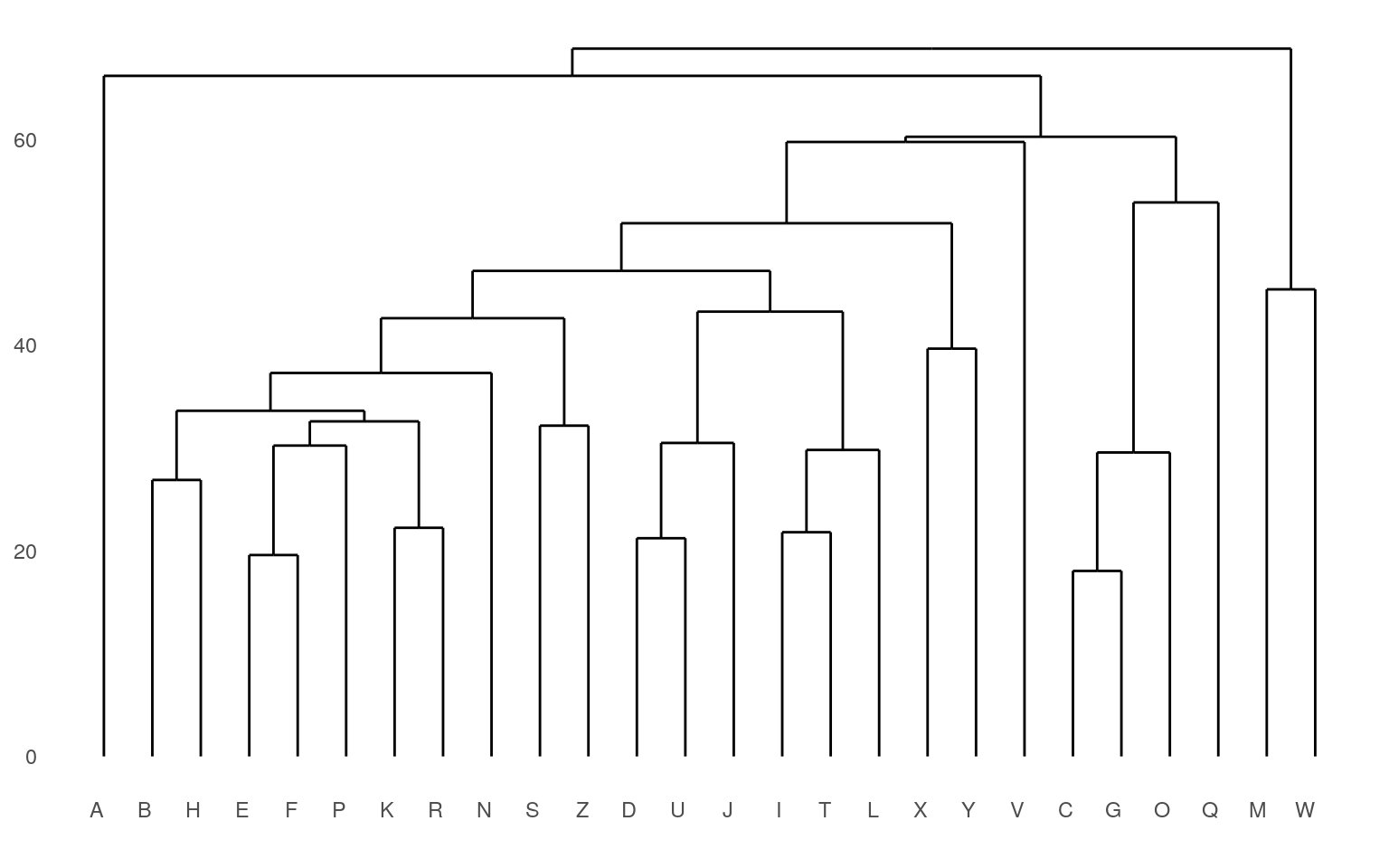
Although agnes can handle a distance matrix, you can also give it a set of feature-values, and it will compute that matrix directly. Remember that these features are developed with a different method than the subjective ratings data we have looked at so far.
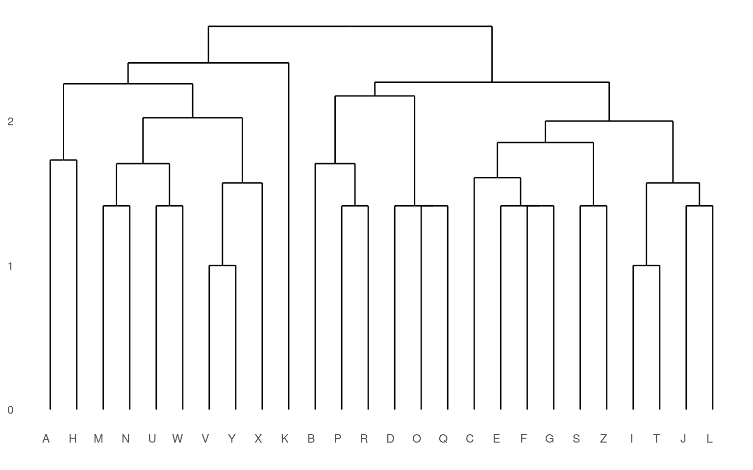
Here, we can see that both clustering solutions capture similar pairs fairly well. Both group E and F together, and put M and W close together. If we look at higher-level clusters, both group round letters together in one group. However, the higher-level structures seem a bit inconsistent. If we wanted to capture the large-scale structure first, we could use a divisive approach; trying to find the best splits from the large-scale data and iteratively dividing.
Divisive Approaches
A second method is to take the entire data set and first find the best way to divide it into two, and then divide those into two, and so on. This is more appropriate if you are more interested in a large-scale class structure. For example, if you had similarity ratings of hundreds of birds, you’d expect birds of the same species to be together at the bottom, but this maybe not as interesting as large-scale divisions (maybe between land and sea birds). In that case, you might consider a divisive approach, which is provided by the diana function.
d <- diana(distmat)
p1 <- ggdendrogram(d)
d2 <- diana(features)
p2 <- ggdendrogram(d2)
grid.arrange(p1, p2, ncol = 2)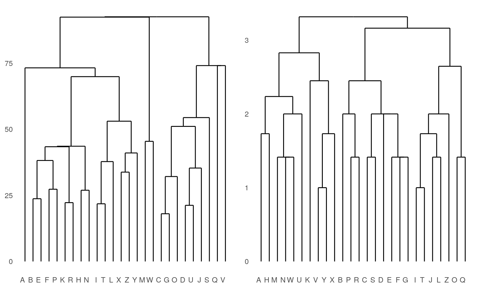
Notice that here, it perhaps does a better job of separating the curved letters from the boxy letters and the letters with diagonals.
Linkage methods of cluster similarity
For agglomerative clustering, the main way to control the outcome is to control how you compute the dissimilarity of a group, or of a group to a new item. These are influnced by the method argument, which can take on values: * single (essentially the distance from the new point to any element of the group) * average (average distance between point and all points in group) * complete (the largest distance from new point to anything in the group) * ward (undocumented) * weighted (some sort of weighted average) * flexible and gaverage (more detailed control)
If we compare some of these alternatives (so far we have used ‘average’, which is the default). In general, these are applicable to both agglomerative and divisive approaches
a2 <- agnes(distmat, method = "single")
a3 <- agnes(distmat, method = "complete")
a4 <- agnes(distmat, method = "ward")
a5 <- agnes(distmat, method = "weighted")

p2 <- ggdendrogram(a2) + labs(title = "Single")

p3 <- ggdendrogram(a3) + labs(title = "Complete")
p4 <- ggdendrogram(a4) + labs(title = "Ward's Method")
p5 <- ggdendrogram(a5) + labs(title = "Weighted")
grid.arrange(p2, p3, p4, p5, ncol = 2)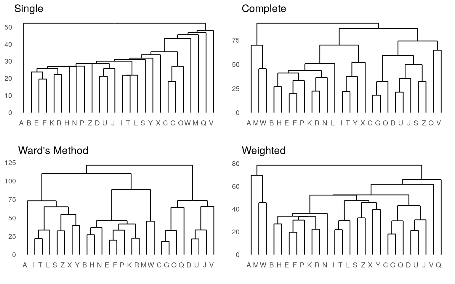
These different methods seem to have large differences in the outcome. The single-linkage model is pretty terrible. This is typical—it sort of links one next-closest item at a time into a chain. Single-linkage models are efficient to calculate because they pick the minimum pairing, but efficiency is not usually a huge concern, and so it is typically not a good idea to use single-linkage. Complete linkage takes the opposite approach, and all of the remaining solutions are pretty reasonable.
Exercise: for the sound-rating data, complete the different clustering methods and linkage methods, and compare the results
## Example:
a.rs <- agnes(features, method = "single")
d.rs <- diana(features)
p1 <- ggdendrogram(a.rs, which = 2)
p2 <- ggdendrogram(d.rs, which = 2)
grid.arrange(p1, p2, ncol = 2)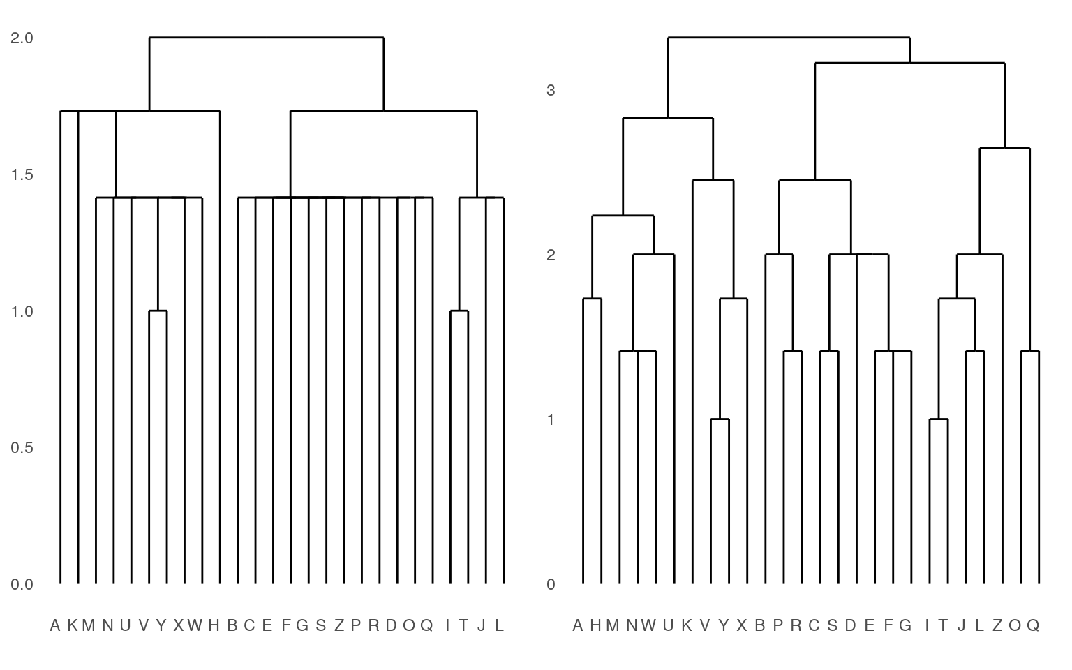 There are some additional clustering methods available within the cluster library, which we will return to as they are more related to k-means clustering.
Finite Clustering Approaches
A second general approach to clustering is to assume a fixed number of clusters exist, and then find the best configuration that matches these clusters. The simplest approach for this is k-means clustering, where \(k\) is the fixed number of clusters. Of course, if we start with a specific value for \(k\), we can obtain a solution and get a measure of the goodness-of-fit. Then, we can compare this solution to solutions provided by other values of \(k\), and try to choose a \(k\) that seems most reasonable.
There are a number of related approaches to this, including finite mixture modeling which we will deal with in a future unit.
K-means clustering
K-means clustering uses distance to define group membership. You specify the number of clusters, and it adaptively sorts observations into clusters, and then adjusts the centers of the clusters to fit the observations. This is easy to implement by hand, but the kmeans function that is part of the R default stats package provides a reasonable solution. One big difference between hierarchical clustering and kmeans clustering is that kmeans requires the ‘raw’ data, not the distance metric, and gives us clusters as defined by the mean values on each feature. If we had just similarity data, we could use MDS to infer features, and then use that inferred space to produce a k-means solution.
Let’s start with a small value for \(k\): say 3.
I J L T Z B C D E F G O P Q R S A H K M N U V W X Y
1 1 1 1 1 2 2 2 2 2 2 2 2 2 2 2 3 3 3 3 3 3 3 3 3 3 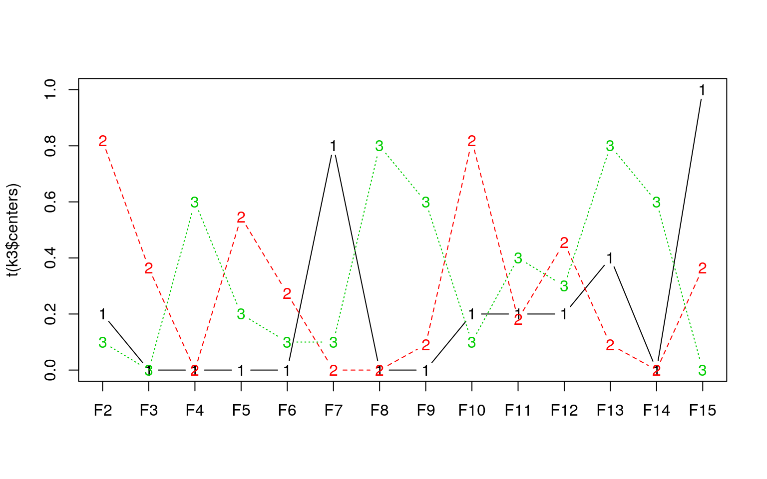
K-means clustering with 3 clusters of sizes 5, 11, 10

Cluster means:
         V2        V3  V4        V5        V6  V7  V8         V9       V10
1 0.2000000 0.0000000 0.0 0.0000000 0.0000000 0.8 0.0 0.00000000 0.2000000
2 0.8181818 0.3636364 0.0 0.5454545 0.2727273 0.0 0.0 0.09090909 0.8181818
3 0.1000000 0.0000000 0.6 0.2000000 0.1000000 0.1 0.8 0.60000000 0.1000000
        V11       V12        V13 V14       V15
1 0.2000000 0.2000000 0.40000000 0.0 1.0000000
2 0.1818182 0.4545455 0.09090909 0.0 0.3636364
3 0.4000000 0.3000000 0.80000000 0.6 0.0000000

Clustering vector:
A B C D E F G H I J K L M N O P Q R S T U V W X Y Z
3 2 2 2 2 2 2 3 1 1 3 1 3 3 2 2 2 2 2 1 3 3 3 3 3 1

Within cluster sum of squares by cluster:
[1]  5.20000 19.45455 20.10000
 (between_SS / total_SS =  38.0 %)

Available components:

[1] "cluster"      "centers"      "totss"        "withinss"
[5] "tot.withinss" "betweenss"    "size"         "iter"
[9] "ifault"
Here, each cluster is defined by the means on 14 dimensions. The solution is as follows:
I J L O Q T Z B C D E F G P R S A H K M N U V W X Y
1 1 1 1 1 1 1 2 2 2 2 2 2 2 2 2 3 3 3 3 3 3 3 3 3 3
K-means provides a goodness of fit statistic, indicating the sum of squares by cluster. By dividing between-group sum-of-squares by within-group, you can figure out the proportion of variance accounted for within versus between clusters. What happens to this when we look at different k-values?
Exercise: do a k-means clustering on the feature-based letter data, exploring the solutions and the sum-of-squares statistics.
Here is a starting point:
k2 <- kmeans(features, centers = 2)
k3 <- kmeans(features, centers = 3)
k4 <- kmeans(features, centers = 4)
k5 <- kmeans(features, centers = 5)
k10 <- kmeans(features, centers = 10)

k2$betweenss/k2$totss
[1] 0.2614739[1] 0.3797344[1] 0.4598183[1] 0.5152554[1] 0.7482232Here, the between/within rises from 26% to 73% as the number of groups goes up to 10. That is, 95% of the total variance is being explained by differences between groups. We’d prefer a smaller proportion, because that means a strong similarity within group and dissimilarity across groups. Here, we also notice a diminishing return for adding more clusters after 4 or 5. Maybe we want to look at the k5 solution:
C D E F G L S A H M N U W B P R I J O Q T Z K V X Y
1 1 1 1 1 1 1 2 2 2 2 2 2 3 3 3 4 4 4 4 4 4 5 5 5 5
This seems a bit better than the 3-cluster solution, as it tends to group together smaller sets of roughly-similar letters.
Fuzzy clustering (FANNY)
Fanny clustering (in the cluster library) is sort of a fuzzy k-means, because each observation may have likelihood of belonging to several clusters. This is not exactly partitioning, but can be helpful in determining how well different observations fit into different clusters.
We will use the feature data for this, examining just three clusters. Let’s use manhattan metric, because these are binary features. Also, initial solutions were poor, and fanny recommended changing the default memb.exp value, which appears to be a sort of soft-max coefficient value.
Fuzzy Clustering object of class 'fanny' :
m.ship.expon.      1.2
objective     44.07947
tolerance        1e-15
iterations          24
converged            1
maxit              500
n                   26
Membership coefficients (in %, rounded):
  [,1] [,2] [,3]
A   90    7    3
B    0  100    0
C    0   96    4
D    0  100    0
E    0   92    8
F    0   98    1
G    0   99    1
H   99    1    0
I    0    0  100
J    0    0  100
K   56   37    7
L    0    0  100
M  100    0    0
N  100    0    0
O   11   75   14
P    0  100    0
Q    1   92    7
R    2   97    1
S    0   81   19
T    0    0  100
U   97    2    2
V  100    0    0
W  100    0    0
X  100    0    0
Y   94    0    5
 [ reached getOption("max.print") -- omitted 1 row ]
Fuzzyness coefficients:
dunn_coeff normalized
  0.912930   0.869395
Closest hard clustering:
A B C D E F G H I J K L M N O P Q R S T U V W X Y Z
1 2 2 2 2 2 2 1 3 3 1 3 1 1 2 2 2 2 2 3 1 1 1 1 1 3

Available components:
 [1] "membership"  "coeff"       "memb.exp"    "clustering"  "k.crisp"
 [6] "objective"   "convergence" "diss"        "call"        "silinfo"
[11] "data" 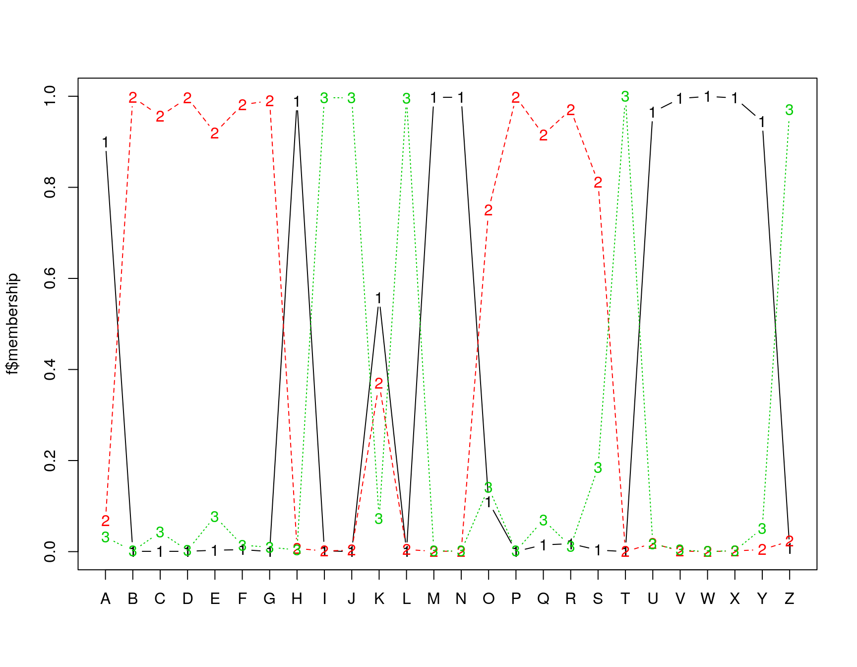
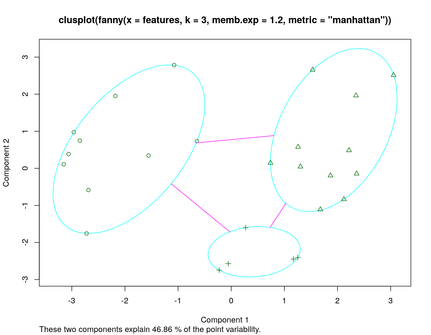
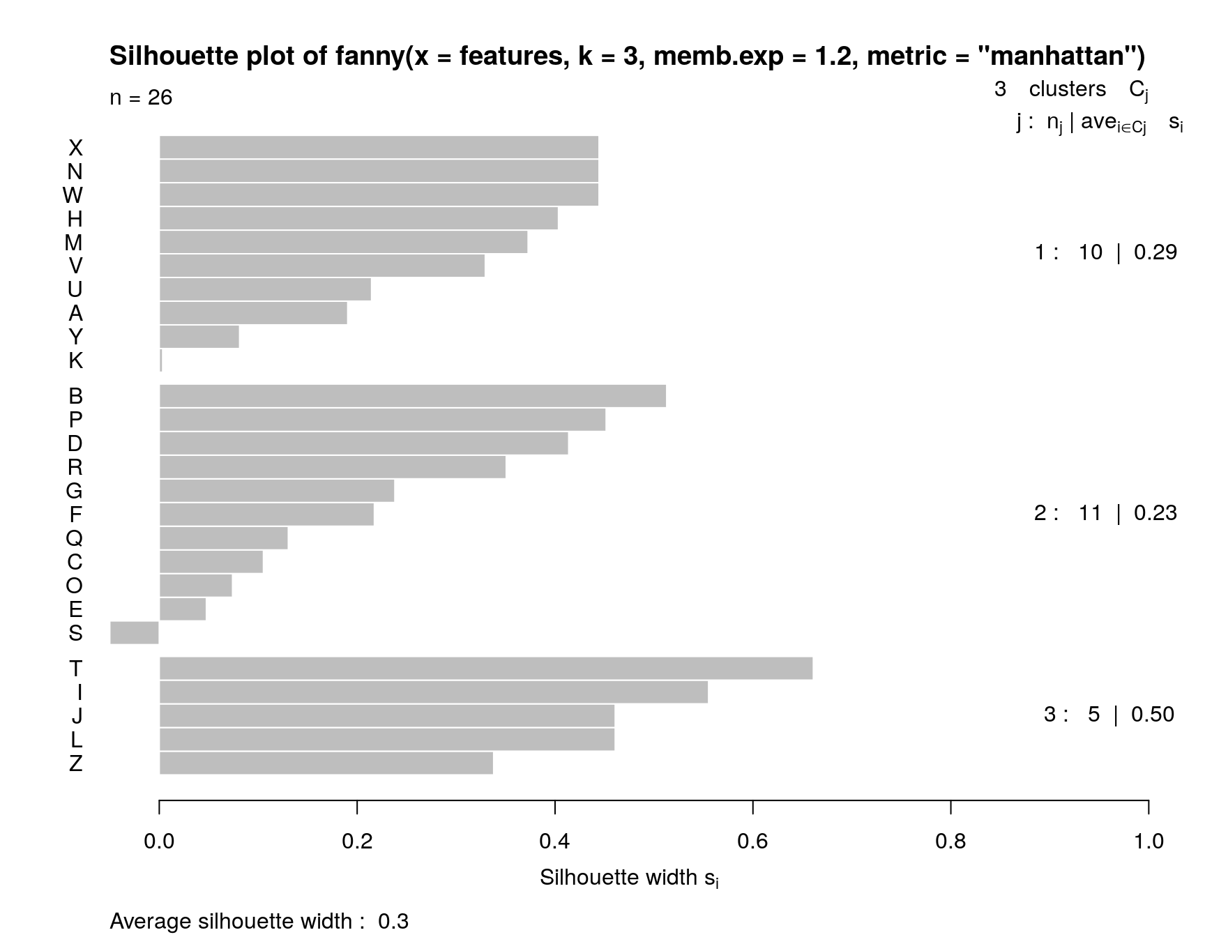
In this analysis, we have assumed three clusters. The matplot we performed returns a membership value, which indicates a fuzzy membership level in each of the clusters. Some values are unambiguous (M and N), but others are less so, (like K). If we then place the item in the best group, we can get a measure of how well it fits that group using a silhouette plot. The horizontal width of the silhouette plot shows how well each item is described by the cluster it ended up in. Sometimes, a few elements will fall ‘below the waterline’, meaning that they are not well described by the cluster they are placed in. For example, K and S are poor. According to the fuzzy membership number, although K is most likely to be in group 1, it is about equally likely to be in either group 3 or 2.
Fanny also returns some fuzzyness coefficients that indicate how well the model works (the dunn coefficient). This might be used to compare to other choices of k.
Exercise: Do a fanny clustering for different k-sizes and compare results.
Partition around Mediods (PAM)
The PAM clustering approach (also in the cluster library) assumes a fixed number of ‘mediods’ that you specify. These mediods are like centroids, but are exemplars that are in the data, rather than a ‘prototype’ or average mixture of all of the elements in that group. Like agnes and diana, pam can use either a distance matrix or raw data (in which case you need to specify the metric.). It also provides a silhouette plot. Let’s look at the original letter data, with k=2,3, and 4:
p2 <- pam(distmat, k = 2)
p3 <- pam(distmat, k = 3)
p4 <- pam(distmat, k = 4)
par(mfrow = c(1, 3))
plot(p2)
plot(p3)
plot(p4)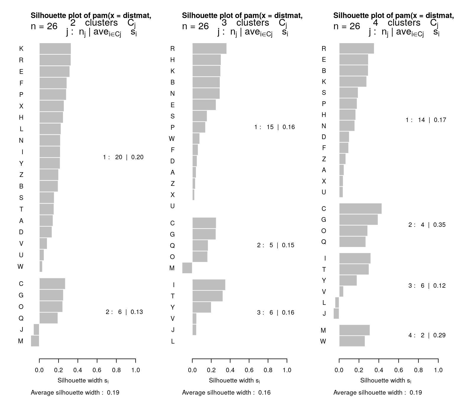
Medoids:
     ID
[1,] "5"  "E"
[2,] "3"  "C"
[3,] "9"  "I"
[4,] "23" "W"
Clustering vector:
A B C D E F G H I J K L M N O P Q R S T U V W X Y Z
1 1 2 1 1 1 2 1 3 3 1 3 4 1 2 1 2 1 1 3 1 3 4 1 3 1
Objective function:
   build     swap
28.65732 28.65732

Available components:
[1] "medoids"    "id.med"     "clustering" "objective"  "isolation"
[6] "clusinfo"   "silinfo"    "diss"       "call"
These again show a goodness of fit between each point in a cluster and all other points in that cluster. Note that they rank order the observations in each based on the silhouette width, which is sort of a typicality of the observation. Usually, the mediod has the highest silhouette value, but not always. For example, for k=4, the mediods were E, C, I, and W. The silhouette plot is not showing the exact values used to make the clustering, (distance to mediod), but rather an overall average similarity. Negative values indicate poor fit, and may mean more clusters are needed.
PAM is interesting beceause it uses just the similarity values. It does not need to recompute any similarities. It also gives a center item that can be used to label the group–rather than considering an arbitrary point in an arbitrary space. But it requires the similarity or distance metric, whose size is \(n*(n-1)/2\). This can get large as the data set gets large, and so may get inefficient.
clara: PAM with a lot of data
If you have a lot of data, the similarity matrix is the square of the number of elements, and it can get very large, and these methods can grow very inefficient. the clara function handles larger data sets. Instead of using a complete dissimilairty matrix, it instead takes a set of features. We can use the big five data set to illustrate this. If we want to identify clusters of people, with 1,000+ people, that would be more than 1,000,000 pairings. Let’s consider the big-five data set, which had 1017 participants:
data <- read.csv("bigfive.csv")

dat.vals <- data[, -1]  ##remove subject code
dat.vals[is.na(dat.vals)] <- 3
qtype <- c("E", "A", "C", "N", "O", "E", "A", "C", "N", "O", "E", "A", "C",
    "N", "O", "E", "A", "C", "N", "O", "E", "A", "C", "N", "O", "E", "A", "C",
    "N", "O", "E", "A", "C", "N", "O", "E", "A", "C", "N", "O", "O", "A", "C",
    "O")
valence <- c(1, -1, 1, 1, 1, -1, 1, -1, -1, 1, 1, -1, 1, 1, 1, 1, 1, -1, 1,
    1, -1, 1, -1, -1, 1, 1, -1, 1, 1, 1, -1, 1, 1, -1, -1, 1, -1, 1, 1, 1, -1,
    1, -1, 1)
add <- c(6, 0, 0)[valence + 2]


tmp <- dat.vals
reversed <- t(t(tmp) * valence + add)
## reverse code questions:
bytype <- reversed[, order(qtype)]
key <- sort(qtype)
colnames(bytype) <- paste(key, 1:44, sep = "")
Let’s do a clara clustering by people–which might be needed because we have so many people observed.
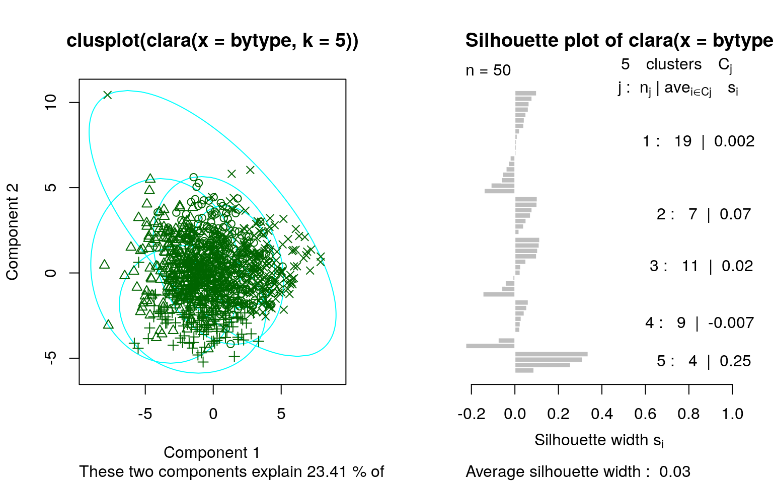
     size  max_diss  av_diss isolation
[1,]  323 11.661904 7.502126  1.971222
[2,]  259 11.747340 7.633261  1.985663
[3,]  185 11.000000 7.799525  1.697337
[4,]  212 15.620499 7.313189  2.501282
[5,]   38  9.380832 7.292022  1.383128
This suggests that although the big-5 defines up to 2^5=32 personality types, most people fall into just a few (4-5) personality clusters. The largest, group-1, has 323 people in it, which is about 1/3 of the data. If we look at the mediod, it is a set of answers across the entire data survey:
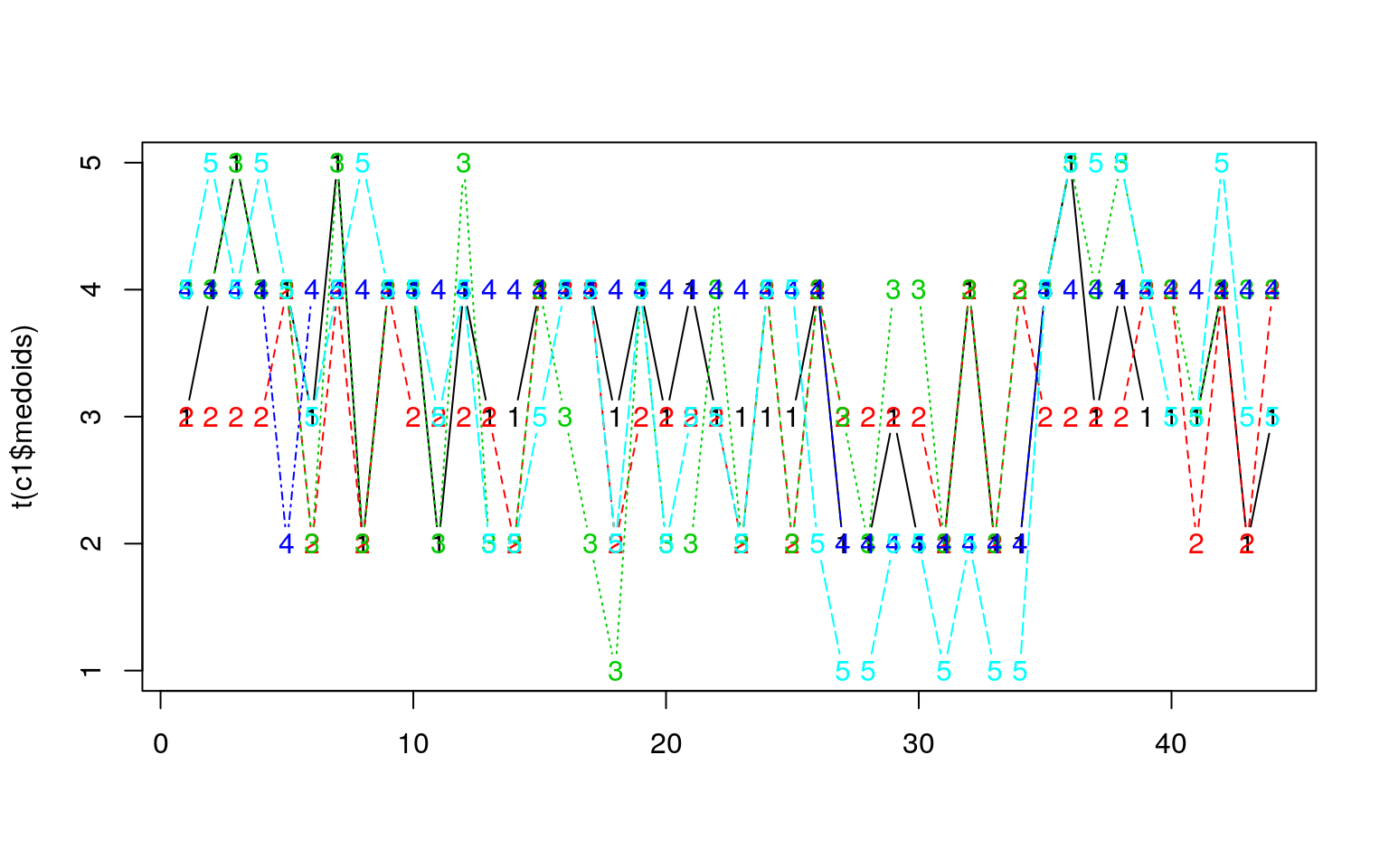
Each series is a person who best describes one group, across the 44 questions of the survey.
Cluster by question:
Since there were five cluster types, maybe we can use this to cluster by question. We will use clara again, although now there are 1000+ features and 44 items. It might be better to cluster
c2 <- clara(t(bytype), k = 5)

for (i in 1:5) {
    cat(paste("Group ", i, ":  \n", sep = ""))
    print(c2$clustering[c2$clustering == i])
}
Group 1:
A1 A6 A8 C11 C13 C14 C18
1 1 1 1 1 1 1
Group 2:
A2 A3 A4 A5 A7 A9 C10 C12 C15 C16 C17 O36
2 2 2 2 2 2 2 2 2 2 2 2
Group 3:
E19 E20 E23 E25 O41
3 3 3 3 3
Group 4:
E21 E22 E24 E26 O35 O37 O38 O39 O40 O42 O43 O44
4 4 4 4 4 4 4 4 4 4 4 4
Group 5:
N27 N28 N29 N30 N31 N32 N33 N34
5 5 5 5 5 5 5 5 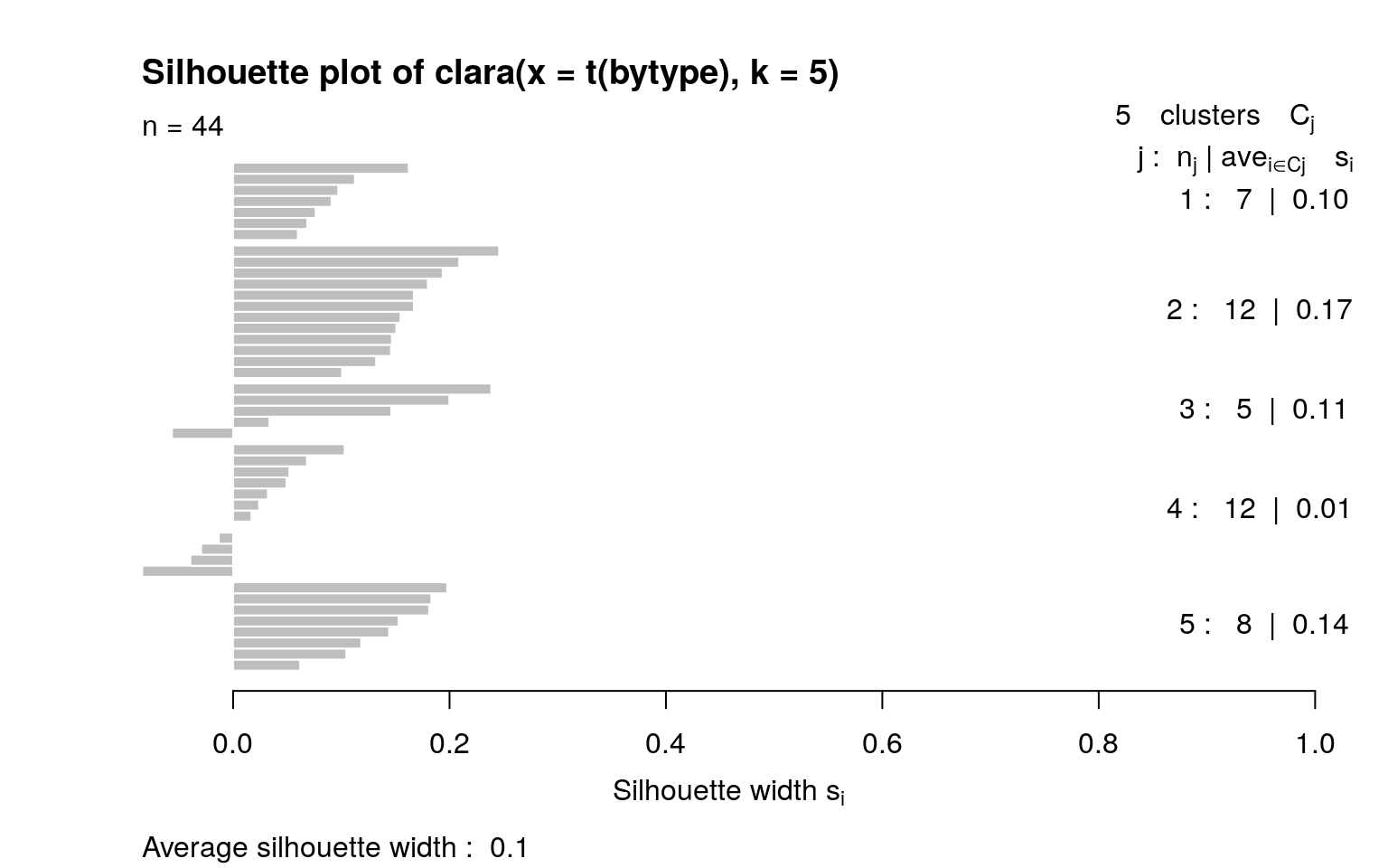
[1] "Cluster membership by personality dimension:"
    1 2 3 4 5
  A 3 6 0 0 0
  C 4 5 0 0 0
  E 0 0 4 4 0
  N 0 0 0 0 8
  O 0 1 1 8 0
Notice that the clusters it picked out were not exactly the 5-dimensions. Part of this may be because of reversed-framed items might not be exactly symmetric with positively-framed questions, but it does suggest that the personality story seems to depend on the method we use to analyze the data.