Model-Based Clustering and mclust
Model-Based Clustering
The previous clustering methods used distance as a means of assessing similarity and forming clusters. This makes intuitive sense, but it would be nice to take a more statistical approach. To do so, we would like to consider a model that might have generated the data. We might assume that the data arose from some distribution (e.g., one or more normal distributions), and try to model the data based on this model. This, in general, is called Model-based clustering. If we make assumptions about the model that generated the data, (and our assumptions happen to be correct), we can perhaps get better classification and clustering.
To do this, we will no longer use distance measures, but work with a set of dimensional or feature data. Otherwise, model-based clustering is much like the algorithm we use to fit k-means clustering, except it works on likelihood instead of distance. Notice how this is the same shift that we underwent earlier in the year, when we moved from least-squares fitting of regression to maximum likelihood.
Let’s start with a 2D example. We will assume that data are generated from a two-dimensional guassian process. Here is an example where, within those two dimensions, our data were generated from three groups with different means, but the same standard deviation:
set.seed(100)

centers <- matrix(runif(6),ncol=3)
par(mfrow=c(1,2))

data1 <- matrix(c(rnorm(200,mean=centers[,1],sd=.02),
              rnorm(200,mean=centers[,2],sd=.02),
              rnorm(200,mean=centers[,3],sd=.02)),

                ncol=2,byrow=T)
colnames(data1) <- c("V1","V2")

plot(data1,col=rep(c("red","darkgreen","blue"),each=100))
points(t(centers),pch=16,cex=2,col="black")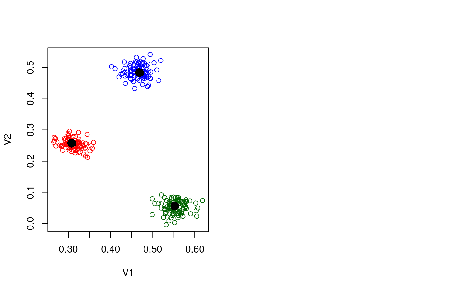
Here, the groups do not overlap at all, but we might imagine a setup where they do:
data2 <- matrix(c(rnorm(200, mean = centers[, 1], sd = 0.1), rnorm(200, mean = centers[,
    2], sd = 0.1), rnorm(200, mean = centers[, 3], sd = 0.1)), ncol = 2, byrow = T)

colnames(data2) <- c("V1", "V2")
plot(data2, col = rep(c("red", "darkgreen", "blue"), each = 100))
points(t(centers), pch = 16, cex = 2, col = c("red", "darkgreen", "blue"))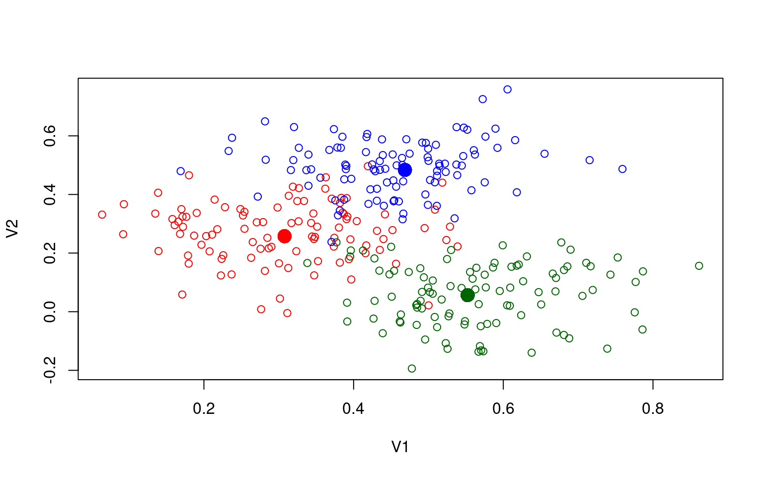
Suppose we assumed the data were from three gaussian distributions, and happened to know the centers of these three distributions, but we don’t know which point came from which distribution. We could estimate the likelihood of each point having come from each of the three groups (each one defined by our estimate of the mean and standard deviation estimate for that group), and use this to help us determine the group it should have belonged to. To do this, we will just use the multivariate density function from the mvtnorm package. We will compute the likelihood of each point for all three models–first for the low-noise data. Here we will do it for data1, which is the most easily discriminable:
library(mvtnorm)
truth <- rep(1:3, each = 100)
center1like <- dmvnorm(data1, mean = centers[, 1], sigma = diag(rep(0.02, 2)))
center2like <- dmvnorm(data1, mean = centers[, 2], sigma = diag(rep(0.02, 2)))
center3like <- dmvnorm(data1, mean = centers[, 3], sigma = diag(rep(0.02, 2)))

likes <- cbind(center1like, center2like, center3like)
group <- apply(likes, 1, which.max)
matplot(cbind(center1like, center2like, center3like), ylab = "Likelihood of each group")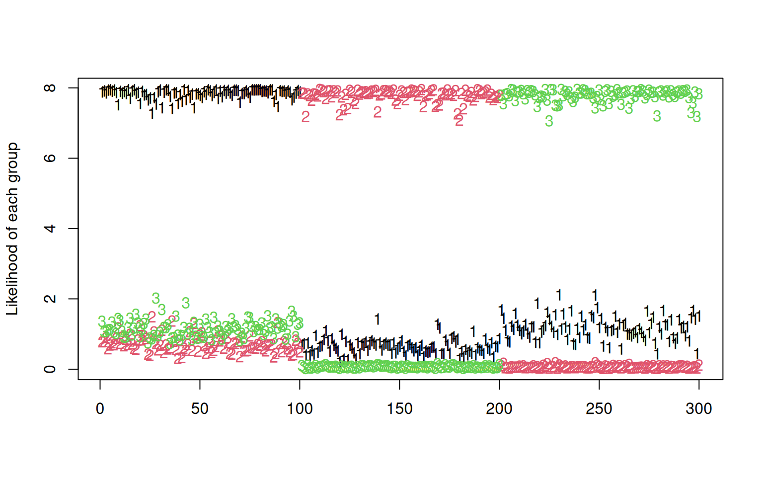
library(ggplot2)
data.frame(data1, original = rep(c("1", "2", "3"), each = 100)) |>
    ggplot(aes(x = V1, y = V2, color = factor(group), shape = original)) + geom_point(size = 3) +
    geom_point(data = as.data.frame(t(centers)), aes(x = V1, y = V2), color = "black",
        size = 5, shape = 4) + theme_bw()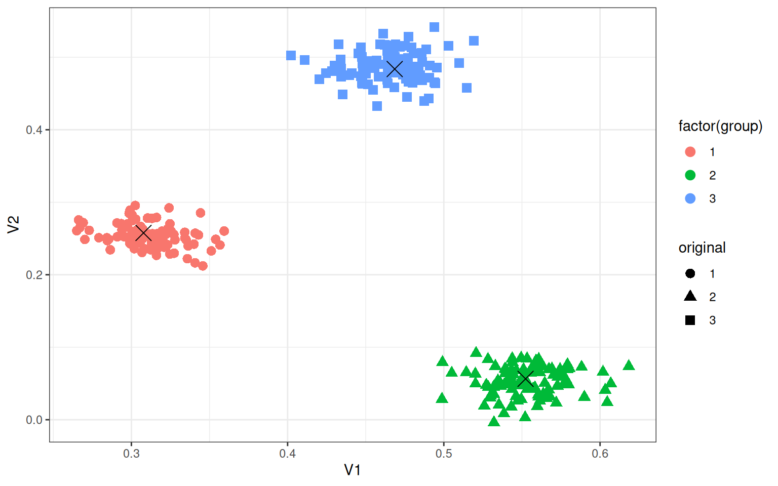
     group
truth   1   2   3
    1 100   0   0
    2   0 100   0
    3   0   0 100
Notice that the points were sampled in sets of 100, and the likelihood model correctly predicts every point if we categorize by the maximum likelihood group. We can look at the high-noise group data2, and it still looks promising, but there might be some errors. So if we knew what the groups looked like, we can in this case correctly classify each member–this is not too different from LDA or other classifiers we examined earlier.
Let’s look at data2, which has more overlap between groups. Again, we will assume we know what each group looks like, and determine, for each data point, the likelihood of the point given each group:
center1like <- dmvnorm(data2, mean = centers[, 1], sigma = diag(rep(0.07, 2)))
center2like <- dmvnorm(data2, mean = centers[, 2], sigma = diag(rep(0.07, 2)))
center3like <- dmvnorm(data2, mean = centers[, 3], sigma = diag(rep(0.07, 2)))
likes <- cbind(center1like, center2like, center3like)

matplot(likes)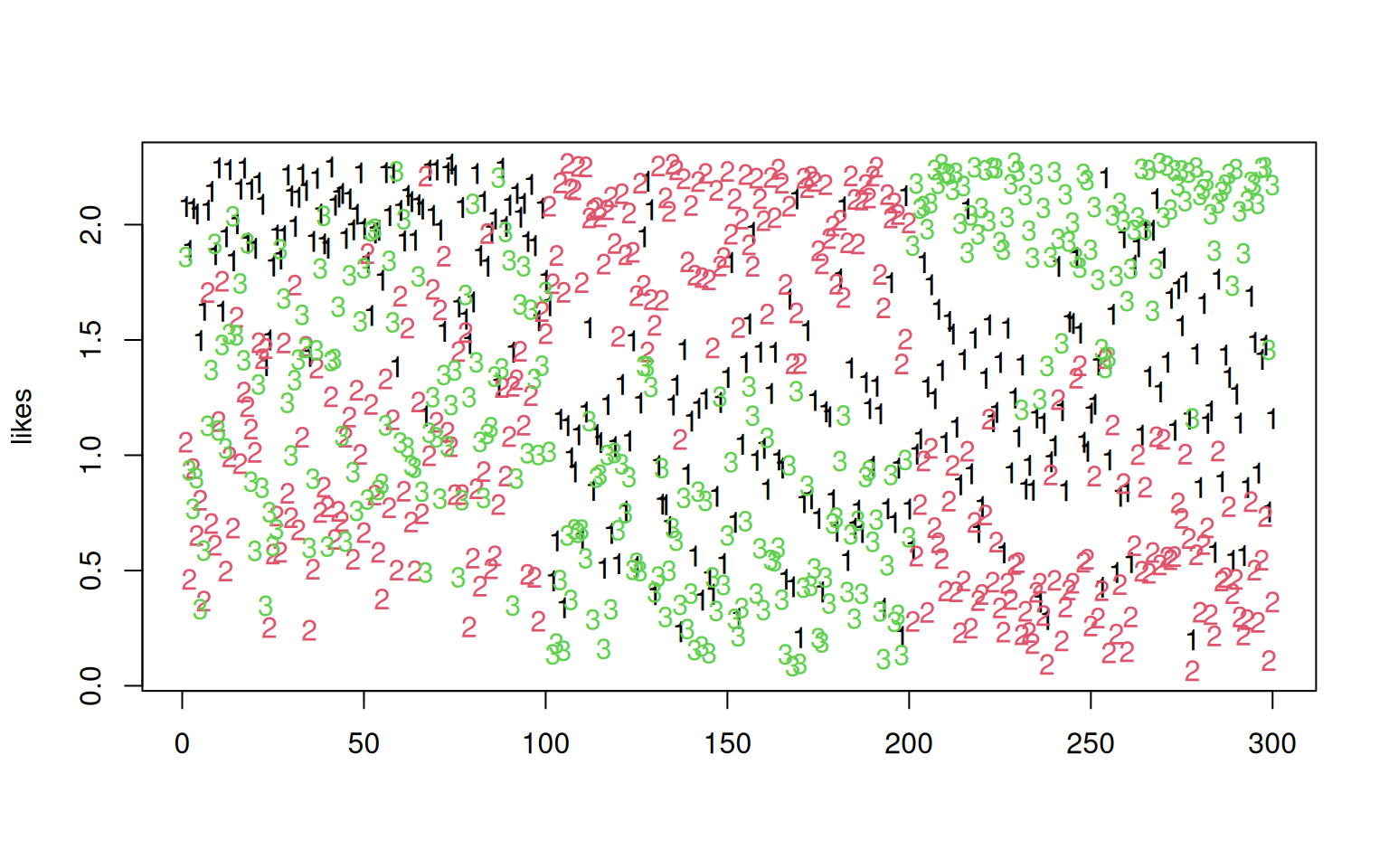
     group
truth  1  2  3
    1 83  6 11
    2  7 93  0
3 6 0 94library(ggplot2)
data.frame(data2, original = rep(c("1", "2", "3"), each = 100)) |>
ggplot(aes(x = V1, y = V2, color = factor(group), shape = original)) + geom_point(size = 3) +
geom_point(data = as.data.frame(t(centers)), aes(x = V1, y = V2), color = "black",
size = 5, shape = 4) + theme_bw()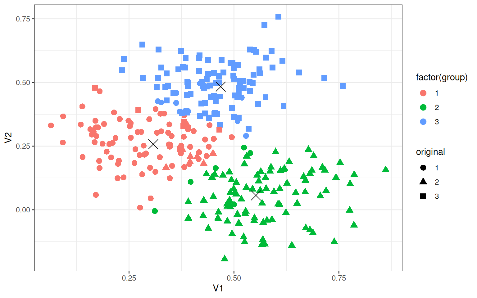
# plot(data2,col=c('red','darkgreen','blue')[group],pch=rep(c(1,16,11),each=100))
# points(t(centers),pch=16,cex=2,col=c('red','darkgreen','blue'))
Looking at the confusion table, this is not perfect, but still very good–around 90% accurate, even though we didn’t know the group membership to start with. The figure shows the original group as shape and the classified group as color, and what was originally overlapping groups are cleanly separated (incorrectly).
However, the caveat is we had the exact description of each true group (which we normally do not have). So, If we know that the data are generated from a normal distribution, and if we assume the variance is the same in both dimensions, and if we know the means of the groups, and if we are right about there being three groups, in many conditions we can do very well at recovering the group structure. The general problem is referred to as model-based clustering, because (unlike earlier clustering approaches), we are modeling each group as a probability distribution. Because we treat the data as being generated by a mixture of unknown sources, this is also called ‘mixture modeling’.
Finite mixture modeling
One common variety of this solution works similarly to k-means clustering, and is referred to as finite mixture modeling. Finite refers to assumptions about how many groups we have, and mixture modeling refers to the mixture of distributions assumptions. Unlike k-means (and more like fanny), finite mixture modeling will permit each item to have a likelihood of being a member of each group. We assume that the data are generated from a mixture of hidden distributions, and the number of these is finite.
Mixture modeling makes a lot of sense when thinking about real processes. For example, suppose you have a visual memory task where you are trying to remember the location of an object. On some trials, you remember, but because your memory is fuzzy, you tend to be off by a little bit. On other trials, you don’t pay attention at all, and so guess. This represents a mixture of two processes or strategies, and researchers have used mixture modeling to estimate memory precision separate from guessing.
Inference for FMM–finding where the groups are–can happen in a number of ways. The simplest method uses a technique called Expectation-Maximization (E-M), but Bayesian approaches are also popular. Aside from the method for identifying clusters, the Bayesian approach will typically produce a distribution of solutions, whereas E-M will produce a single maximum-likelihood solution. In addition, many Bayesian approaches have explored infinite mixture models–permitting the model to have as many groups as you need, and letting the Bayesian inference determine the likely number of groups.
E-M works very similarly to the iterative process of k-means. You begin with a random assignment of items to groups. You then perform Expectation step–estimating group parameters via maximum likelihood and likelihoods for the points given the parameters. Then you perform maximization–sorting each group into the cluster that maximized likelihood. You repeat this until the process converges, and statisticians have proved that it converges under many flexible conditions.
Let’s try this by hand, with data2. Do it multiple times and see the different ways it turns out.
group <- sample(1:3, 300, replace = T)
## Repeat the following until it converges:
par(mfrow = c(1, 2))
for (i in 1:6) {
## recompute centers and spread based on these groupings
## (maximum-likelihood estimation)
groupmeans <- aggregate(data2, list(group), mean)[, -1]
groupsd <- aggregate(data2, list(group), sd)
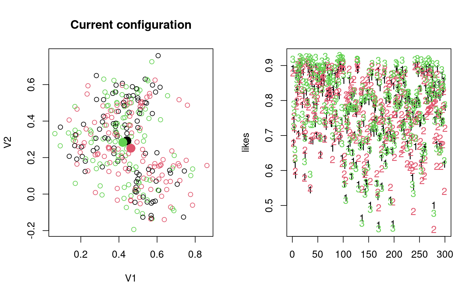
plot(data2, col = group, main = "Current configuration")
points(groupmeans, pch = 16, cex = 2, col = 1:3)
## estimate likelihood for each grouping:
center1like <- dmvnorm(data2, mean = unlist(groupmeans[1, ]), sigma = diag(groupsd[1,
2:3]))
center2like <- dmvnorm(data2, mean = unlist(groupmeans[2, ]), sigma = diag(groupsd[2,
2:3]))
center3like <- dmvnorm(data2, mean = unlist(groupmeans[3, ]), sigma = diag(groupsd[3,
2:3]))
# center2like <-
# dmvnorm(data2,mean=groupmeans[2,],sigma=diag(groupsd[2,2:3])) center3like
# <- dmvnorm(data2,mean=groupmeans[3,],sigma=diag(groupsd[3,2:3]))
likes <- cbind(center1like, center2like, center3like)
matplot(likes)
## redo group assignment
group <- apply(likes, 1, which.max)
print(groupmeans)
print(groupsd)
print(table(truth, group))
}
         V1        V2
1 0.4413749 0.2919114
2 0.4627788 0.2513789
3 0.4204392 0.2832741
  Group.1        V1        V2
1       1 0.1410447 0.2184864
2       2 0.1622768 0.1871675
3       3 0.1414510 0.2076191
     group
truth  1  2  3
    1  0  5 95
    2  0 90 10
    3 31  4 65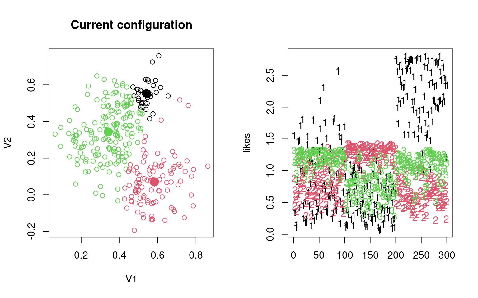
         V1         V2
1 0.5417238 0.55230252
2 0.5820350 0.06969262
3 0.3418263 0.34304246
  Group.1         V1        V2
1       1 0.04294894 0.0743288
2       2 0.09720254 0.1286705
3       3 0.10206785 0.1400391
     group
truth  1  2  3
    1 26  4 70
    2  2 93  5
    3 95  0  5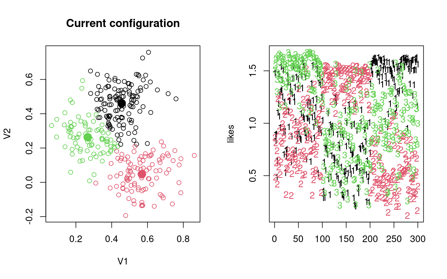
         V1         V2
1 0.4558144 0.46112311
2 0.5686219 0.04752592
3 0.2662983 0.26262512
  Group.1         V1         V2
1       1 0.08832096 0.10774279
2       2 0.10573413 0.09864168
3       3 0.08888657 0.10085525
     group
truth  1  2  3
    1 16  3 81
    2  0 93  7
    3 95  0  5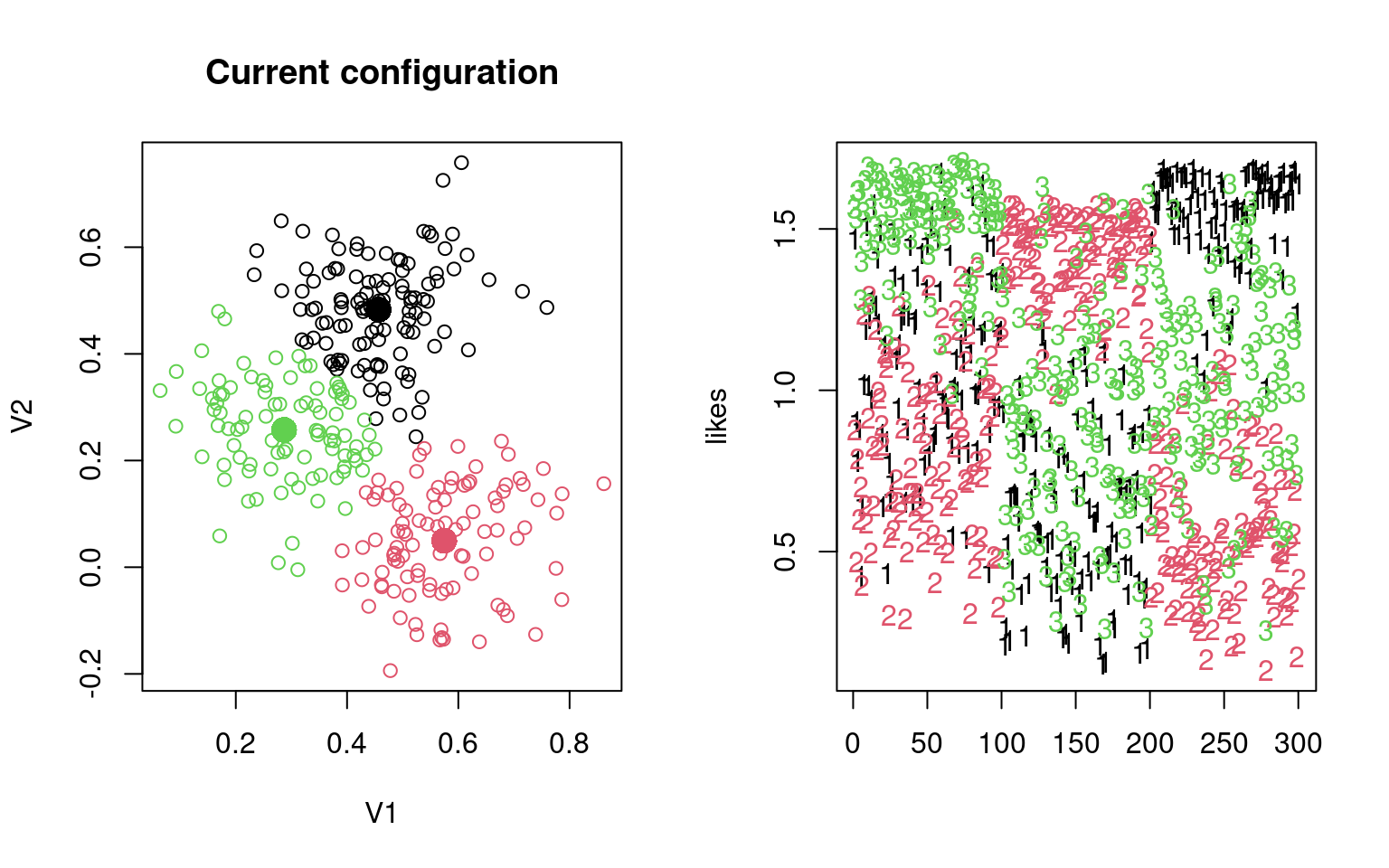
         V1         V2
1 0.4567431 0.48301875
2 0.5745666 0.04970952
3 0.2867580 0.25753732
  Group.1         V1         V2
1       1 0.09323739 0.09534072
2       2 0.10032513 0.10113486
3       3 0.09512524 0.09152437
     group
truth  1  2  3
    1 14  3 83
    2  0 92  8
    3 95  0  5
V1 V2
1 0.4561706 0.48708222
2 0.5767498 0.04961216
3 0.2917868 0.25555259
Group.1 V1 V2
1 1 0.09387153 0.09125792
2 2 0.09918587 0.10255077
3 3 0.09776597 0.09138398
group
truth 1 2 3
1 14 3 83
2 0 92 8
3 95 0 5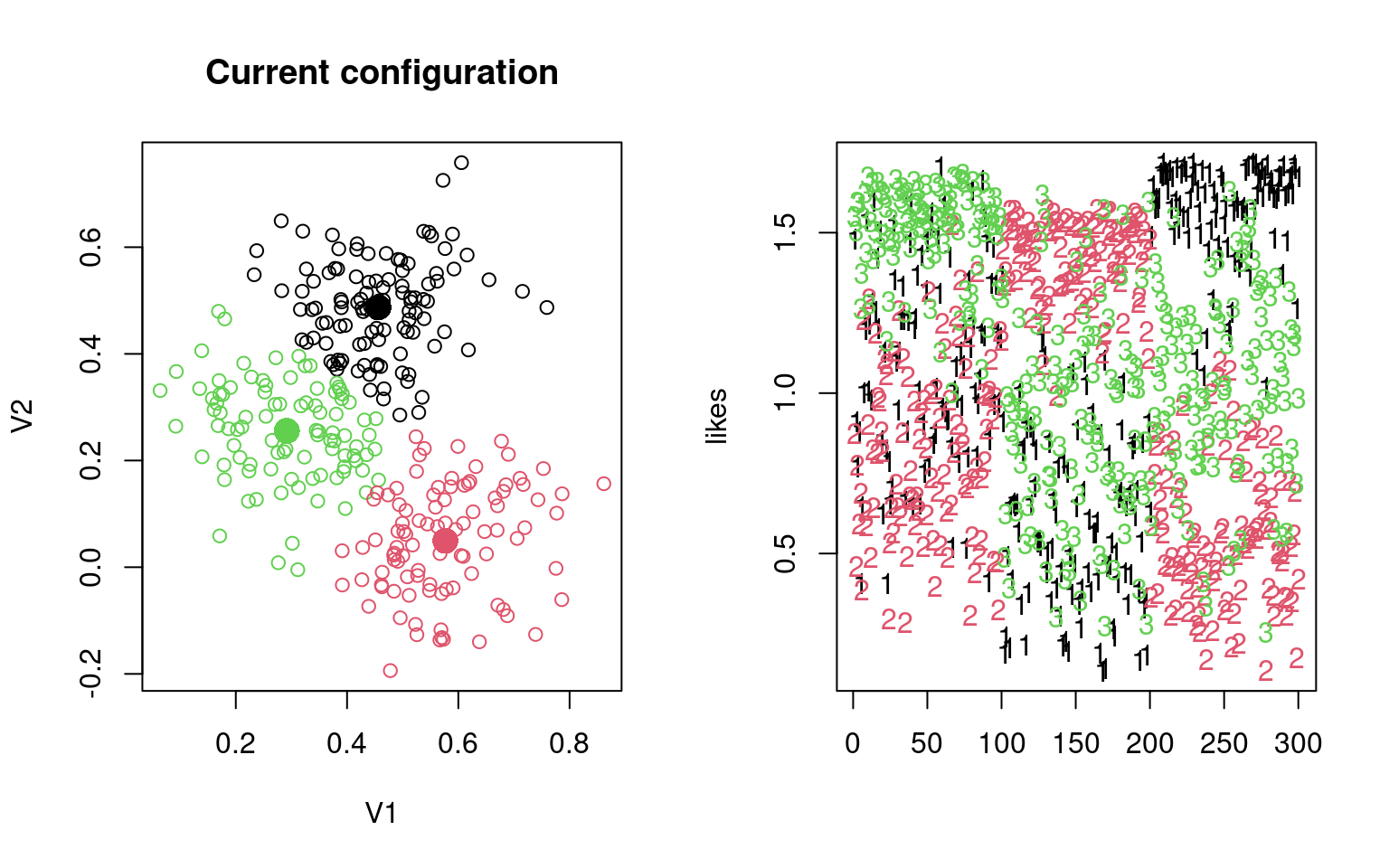
         V1         V2
1 0.4561706 0.48708222
2 0.5767498 0.04961216
3 0.2917868 0.25555259
  Group.1         V1         V2
1       1 0.09387153 0.09125792
2       2 0.09918587 0.10255077
3       3 0.09776597 0.09138398
     group
truth  1  2  3
    1 14  3 83
    2  0 92  8
3 95 0 5 [,1] [,2] [,3]
[1,] 0.3077661 0.55232243 0.4685493
[2,] 0.2576725 0.05638315 0.4837707Notice by looking at the table, that the name of the groups might not be right, but it usually does a good job of categorizing by the fourth round. Sometimes, a group disappears–eaten by another group. We can look at the parameters to identify each model. Note that although the data were created with independence and equal variance, the model estimates the variance of each dimension separately.
The groupsd values should all be around 0.07, which is what generated them. Notice also that the centers are estimated very well.
  Group.1         V1         V2
1       1 0.09387153 0.09125792
2       2 0.09918587 0.10255077
3 3 0.09776597 0.09138398 V1 V2
1 0.4561706 0.48708222
2 0.5767498 0.04961216
3 0.2917868 0.25555259 [,1] [,2] [,3]
[1,] 0.3077661 0.55232243 0.4685493
[2,] 0.2576725 0.05638315 0.4837707We have assumed a normal distribution, which is ``spherical’’, and correctly re-estimated the parameters of that distribution and a hidden piece of information–the group membership. This is how E-M is sometimes used to estimate hidden, latent, or missing information; here the missing information is the group membership variable.
We should also recognize that we have made several assumptions here that might not be true, and perhaps not made others that could have been true. For example:
- Should all groups have the same variability?
- Should a group have the same variability in each direction?
- Should there be covariance, to permit angled ellipses?
Also, we haven’t yet solved the problem of figuring out how many groups there should be. Because we are fitting a likelihood model, likelihood metrics can be used. It is common to use BIC, which will balance model complexity and goodness of fit, to determine how many groups to use.
Finally, if you the solution to the model is going to be very dependent on starting conditions. There is only one ‘best’ solution, but we may not find it unless we run the model a few hundred times from different configurations.
For these reasons, it is usually better to use a built-in library that handles all these issues. the mclust and the flexmix libraries are both very good. We will focus on mclust, which is faster and offers a lot of built-in models. The flexmix library is more flexible, but sometimes requires you to build a model driver by hand. mclust focuses primarily on gaussian mixture modeling, and is very fast.
----------------------------------------------------
Gaussian finite mixture model fitted by EM algorithm
----------------------------------------------------

Mclust EII (spherical, equal volume) model with 3 components:

 log-likelihood   n df      BIC      ICL
       260.7488 300  9 470.1636 399.5207

Clustering table:
  1   2   3
97 104 99 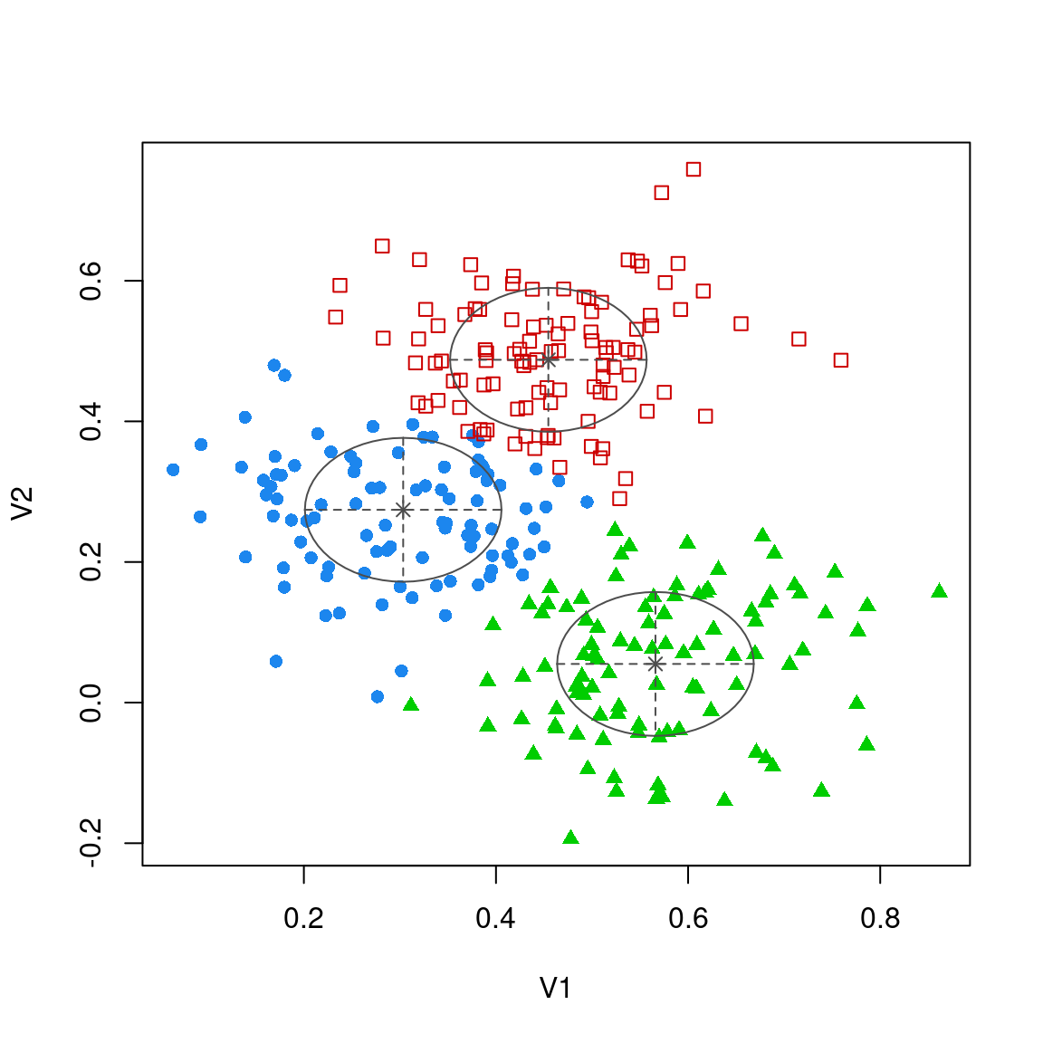
Without asking, this identified that we had three components, showed how many were in each group, and produced likelihood and BIC scores. It also states it used model ‘EII’. Unpacking this, EII refers to the type of guassian variance model. There are many different options. The model actually fit all the different variance options, and compared them via a BIC score to choose the best:
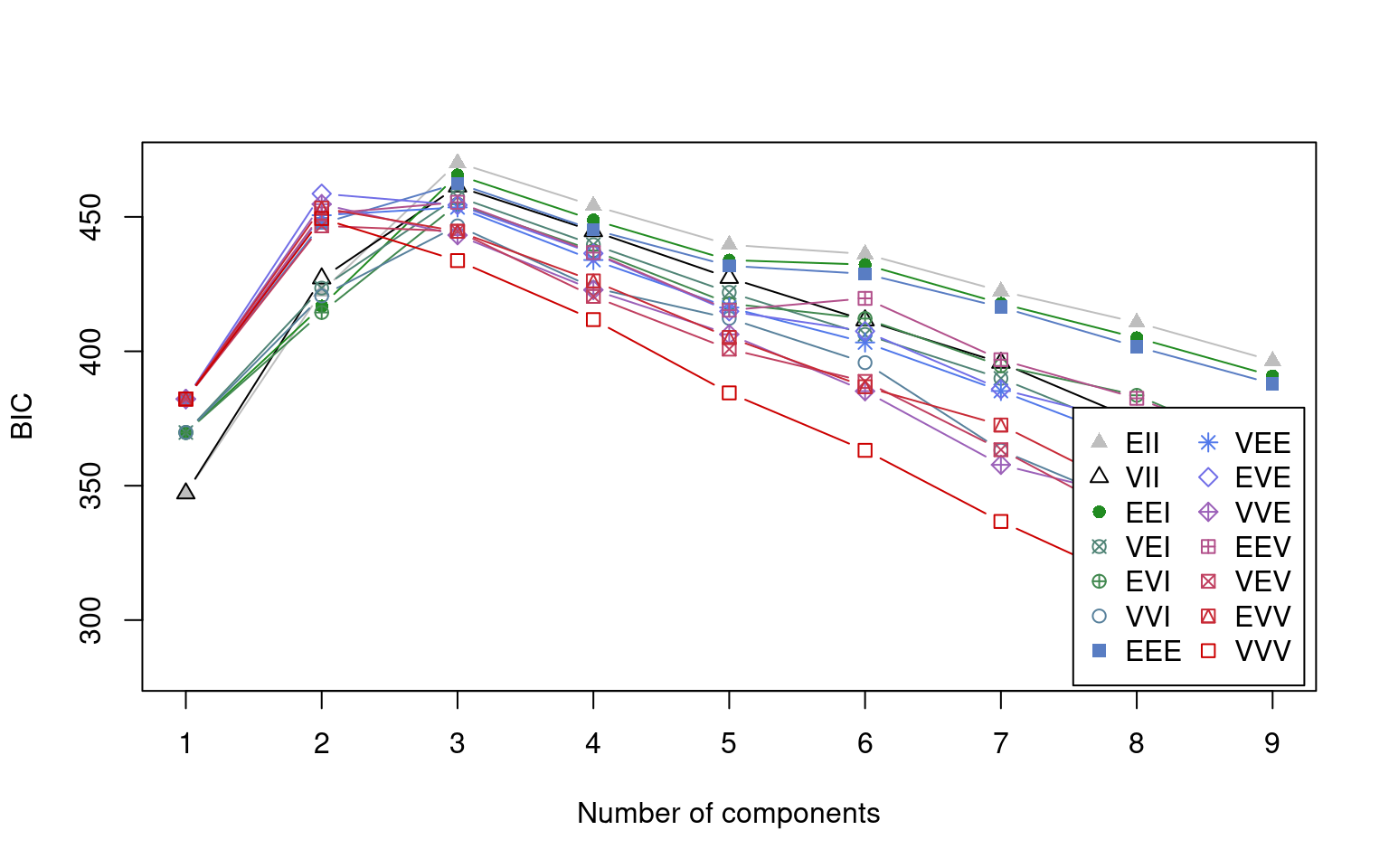
We can see about 14 different models here. In mclust, we are looking for the most positive BIC score, and across models that it 3 components for the EII model. But there are other models we could also choose, and some of those appear to prefer 2 groups. MClust provides a few models that don’t apply to multivariate mixture models as well (“E” and “V”), so if you choose those for a multivariate data set the model might not work. From the help file for mclustModelNames:
The following models are available in package mclust:
univariate mixture
"E"  =   equal variance (one-dimensional)
"V"  =   variable variance (one-dimensional)
multivariate mixture
"EII"    =   spherical, equal volume
"VII"    =   spherical, unequal volume
"EEI"    =   diagonal, equal volume and shape
"VEI"    =   diagonal, varying volume, equal shape
"EVI"    =   diagonal, equal volume, varying shape
"VVI"    =   diagonal, varying volume and shape
"EEE"    =   ellipsoidal, equal volume, shape, and orientation
"EVE"    =   ellipsoidal, equal volume and orientation (*)
"VEE"    =   ellipsoidal, equal shape and orientation (*)
"VVE"    =   ellipsoidal, equal orientation (*)
"EEV"    =   ellipsoidal, equal volume and equal shape
"VEV"    =   ellipsoidal, equal shape
"EVV"    =   ellipsoidal, equal volume (*)
"VVV"    =   ellipsoidal, varying volume, shape, and orientation
single component
"X"  =   univariate normal
"XII"    =   spherical multivariate normal
"XXI"    =   diagonal multivariate normal
"XXX"    =   ellipsoidal multivariate normal
In general, the lower the model, the more complex it is, and so the more parameters needed and the greater improvement needed to justify using it. The model picked EII–spherical equal volume. Spherical indicates the variance is equal in all directions, and equal volume indicates that all variances are assumed to be equal. In contrast to spherical, diagonal would permit each dimension to have a different variance, and ellipsoidal will permit covariance terms to orient the ellipse in different directions. On the other hand, we can constrain aspects of shape and volume (size) across groups, forcing them to be the same or allowing them to differ.
We can see in the parameters how the constraints work out. The variance-sigma values are all identical. The could differ, or we could permit covariance.
$pro
[1] 0.3284201 0.3408899 0.3306900

$mean
        [,1]      [,2]       [,3]
V1 0.3033886 0.4545137 0.56600799
V2 0.2742091 0.4876100 0.05498639

$variance
$variance$modelName
[1] "EII"

$variance$d
[1] 2

$variance$G
[1] 3

$variance$sigma
, , 1

           V1         V2
V1 0.01047352 0.00000000
V2 0.00000000 0.01047352

, , 2

           V1         V2
V1 0.01047352 0.00000000
V2 0.00000000 0.01047352

, , 3

           V1         V2
V1 0.01047352 0.00000000
V2 0.00000000 0.01047352


$variance$Sigma
           V1         V2
V1 0.01047352 0.00000000
V2 0.00000000 0.01047352

$variance$sigmasq
[1] 0.01047352

$variance$scale
[1] 0.01047352
We can force use of another model–for example one with covariance.
----------------------------------------------------
Gaussian finite mixture model fitted by EM algorithm
----------------------------------------------------

Mclust VVI (diagonal, varying volume and shape) model with 3 components:

 log-likelihood   n df      BIC      ICL
       263.2538 300 14 446.6547 383.0861

Clustering table:
  1   2   3
104 95 101 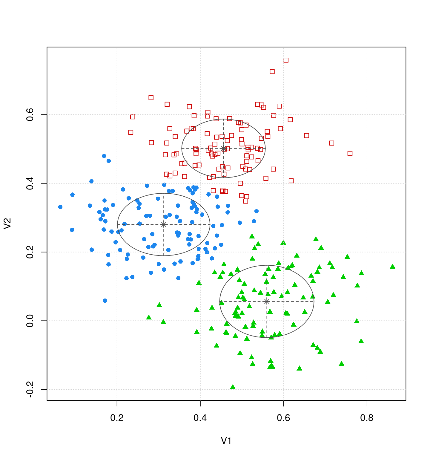
$pro
[1] 0.3429819 0.3174936 0.3395244

$mean
        [,1]      [,2]       [,3]
V1 0.3121680 0.4557030 0.55960752
V2 0.2801813 0.5016499 0.05623381

$variance
$variance$modelName
[1] "VVI"

$variance$d
[1] 2

$variance$G
[1] 3

$variance$sigma
, , 1

           V1          V2
V1 0.01234934 0.000000000
V2 0.00000000 0.008257076

, , 2

           V1          V2
V1 0.01007904 0.000000000
V2 0.00000000 0.007299181

, , 3

          V1         V2
V1 0.0128181 0.00000000
V2 0.0000000 0.01110417


$variance$sigmasq
[1] 0.010097991 0.008577223 0.011930396

$variance$scale
[1] 0.010097991 0.008577223 0.011930396

$variance$shape
             1         2         3
[1,] 1.2229501 1.1750939 1.0744067
[2,] 0.8176949 0.8509958 0.9307462
It did not make much of a difference permitting these to differ. They did change slightly, but values are all very similar across dimensions and groups. We can get the classification response out of the model directly.
truth  1  2  3
    1 83 11  6
    2  7  0 93
    3  7 93  0
truth  1  2  3
    1 85  7  8
    2  7  0 93
    3 12 88  0
Notice that the ‘true’ group membership (which we normally don’t have access to) does not necessarily align with our inferred membership. Because there is no reason why we called our groups 1, 2, and 3, there is also no reason why the model should label the same groups as 1, 2, and 3.
Exercise:
- Build mclust models from the letter-feature data.
- Build mclust models from the personality data.
For each model, select the type of model you feel is most reasonable, and identify how many groups of people/sounds there are. Then, look at the average sound/person from each category and see if there is something that the category captures.
Using mixture modeling with similarity/Distance data
Because mixture modeling works within a dimensional or feature space, the most popular versions will not work if you have a distance measure (like we used for hierarchical clustering). Without developing new algorithms, one way you can still apply tool like Mclust is to use MDS to infer a dimensional space, and then apply finite mixture modeling to that. The choice of k might matter in these cases, but you are not restricted to choosing a 2-dimensional solution. Here is an example using the letter distance data:
library(MASS)
d_dist <- read.csv("plaindist.csv")
d_dist <- d_dist[, -1]
colnames(d_dist) <- LETTERS
rownames(d_dist) <- LETTERS
x <- isoMDS(as.dist(d_dist), k = 3)
initial value 21.183195
iter 5 value 14.763980
iter 10 value 13.824625
iter 10 value 13.812779
iter 10 value 13.807954
final value 13.807954
converged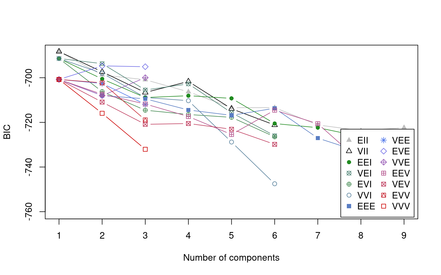
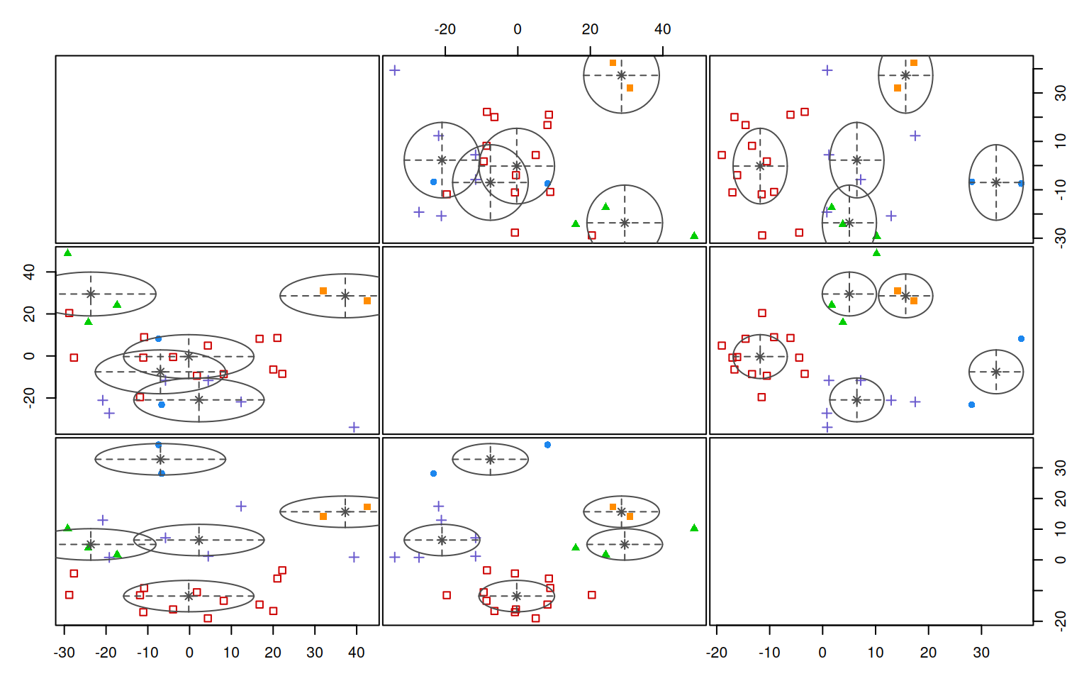
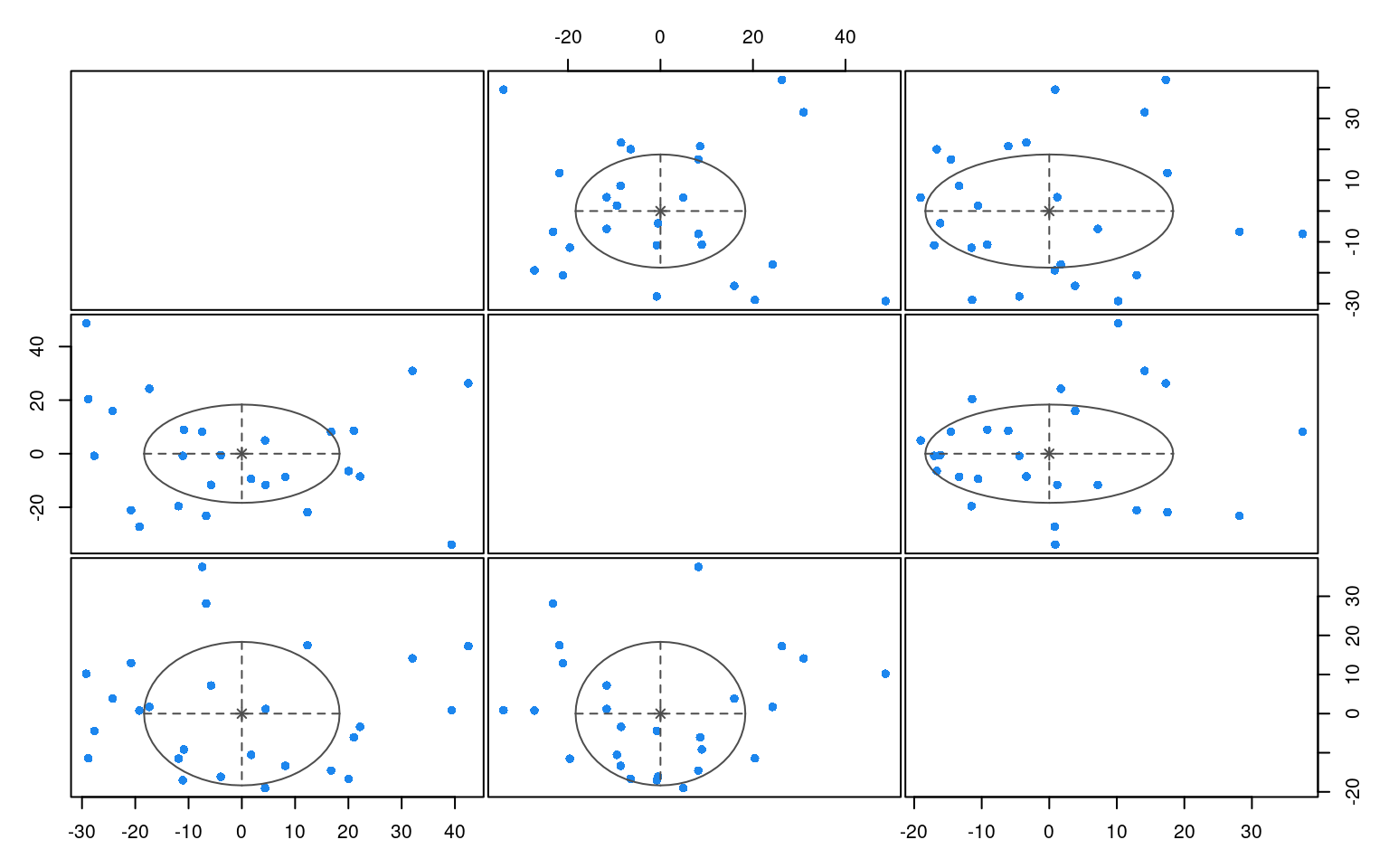 Here, the one-group solution was always the best. Notice that because we
used 3 dimensions, when we plot the mclust solution, it shows us cluster
breakdown for each pair of dimensions.
Here, the one-group solution was always the best. Notice that because we
used 3 dimensions, when we plot the mclust solution, it shows us cluster
breakdown for each pair of dimensions.
Although the algorithms is very similar conceptually to k-means clustering, it has the advantage of giving us a clear criterion for choosing what the best k should be, using the BIC criterion. This criterion balances the number of parameters in the model with the goodness of fit. Here BIC prefers a single solution, because the BIC criterion is very conservative. Part of this is that the BIC incorporates number of observations into its measure. In this case though, we’ve already averaged across our observations, and there may have been dozens of participants and hundreds of trials. Thus, the BIC is probably not really appropriate, because it takes \(N\) as the number of entities we are clustering. We can always force Mclust to use a specified number of cluster if we think that is better than choosing the best via BIC.
 Notice that plotting this will not show the actual letters, but we can
improvise:
Notice that plotting this will not show the actual letters, but we can
improvise:
plot(x$points[, 1], x$points[, 2], type = "n")
text(x$points[, 1], x$points[, 2], LETTERS, col = l5$classification)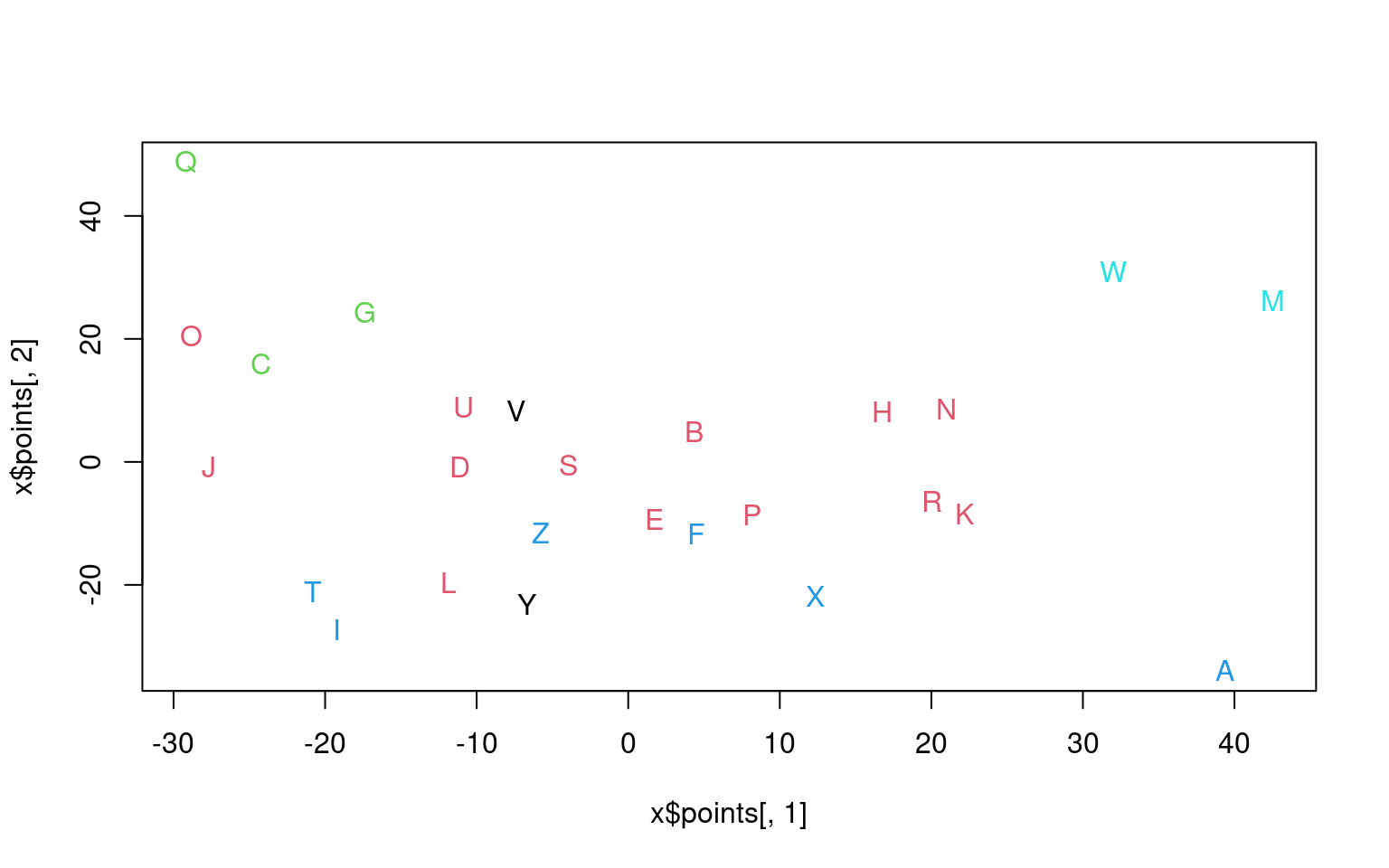
Exercise: Mixture model with personality data
- Use mclust to find clusters of personalities.
- Use mclust to find clusters of personality questions.
data <- read.csv("bigfive.csv")

dat.vals <- data[, -1]  ##remove subject code
qtype <- c("E", "A", "C", "N", "O", "E", "A", "C", "N", "O", "E", "A", "C", "N",
    "O", "E", "A", "C", "N", "O", "E", "A", "C", "N", "O", "E", "A", "C", "N", "O",
    "E", "A", "C", "N", "O", "E", "A", "C", "N", "O", "O", "A", "C", "O")
valence <- c(1, -1, 1, 1, 1, -1, 1, -1, -1, 1, 1, -1, 1, 1, 1, 1, 1, -1, 1, 1, -1,
    1, -1, -1, 1, 1, -1, 1, 1, 1, -1, 1, 1, -1, -1, 1, -1, 1, 1, 1, -1, 1, -1, 1)
add <- c(6, 0, 0)[valence + 2]


tmp <- dat.vals
reversed <- t(t(tmp) * valence + add)
## reverse code questions:
bytype <- reversed[, order(qtype)]
key <- sort(qtype)
colnames(bytype) <- paste(key, 1:44, sep = "")

## we may need to impute missing dat.  If so, a value of 3 is a quick
## reasonable guess:

bytype[is.na(bytype)] <- 3
Hierarchical Model-based Clustering with mclust
mclust also provides a hierarchical model-based clustering. This will still use a limited number of models to characterize a group, but attempt to identify a hierarchical structure. Like normal mclust, hc have varieties hcE, hcV, hcEII, hcVII, hcEEE, hcVVV, that can be specified by modelName.
      2 3 4 5 6 7 8 9 10 11
 [1,] 1 1 1 1 1 1 1 1  1  1
 [2,] 1 1 1 2 2 2 2 2  2  2
 [3,] 1 1 1 2 3 3 3 3  3  3
 [4,] 1 1 1 2 2 2 2 2  2  2
 [5,] 1 1 1 2 3 3 3 3  3  3
 [6,] 1 1 1 2 2 2 2 2  2  2
 [7,] 1 1 1 2 3 3 3 3  4  4
 [ reached getOption("max.print") -- omitted 3 rows ]
This will have N x N-1 matrix, where each column specifies a different level of hierarchical cluster. We can plot each layer consecutively, so you can see how each cluster gets divided.
mc <- Mclust(data2)
hc <- hclass(hh)
par(mfrow = c(2, 2))
plot(data2, col = hc[, 1])
plot(data2, col = hc[, 2])
plot(data2, col = hc[, 5])
plot(data2, col = hc[, 10])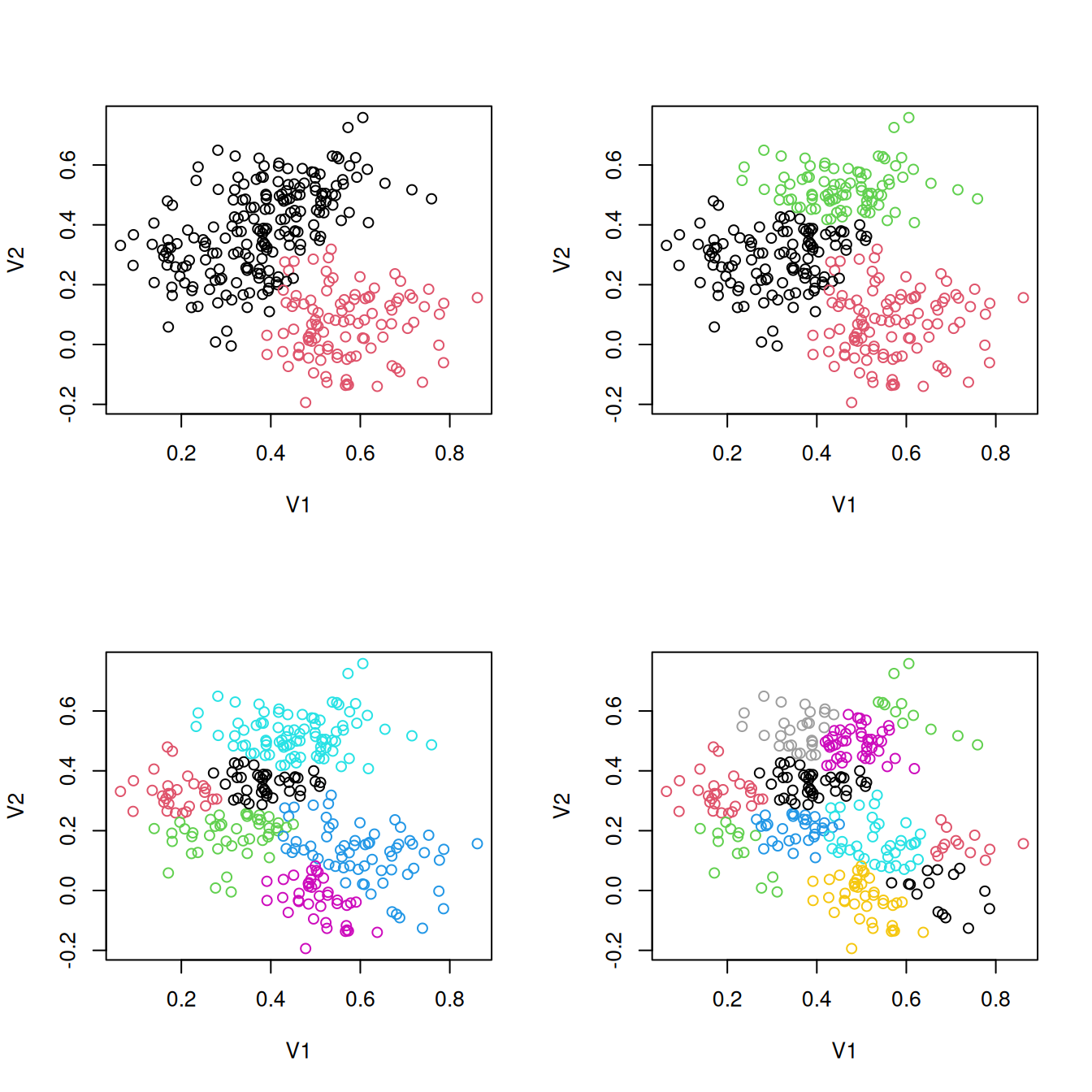
Notice how the clusters are always divided into two clusters. This provides an interesting hybrid approach, and also a means for determining how deeply to cluster–using the BIC criterion
Bayesian Information Criterion (BIC):
        EII       VII       EEI       VEI       EVI       VVI
1 -6136.664 -6136.664 -5261.581 -5261.581 -5261.581 -5261.581
2        NA        NA        NA        NA        NA        NA

Top 3 models based on the BIC criterion:
    EEI,1     EVI,1     VEI,1
-5261.581 -5261.581 -5261.581 Bayesian Information Criterion (BIC):
EII VII EEI VEI EVI VVI EEE
1 -959184.0 -959184.0 -881899.3 -881899.3 -881899.3 -881899.3 -464331.8
2 -860096.4 -860644.8 -792954.2 -788562.5 -792931.7 -788975.1 NA
3 -811788.0 -807346.9 -751240.1 -749064.6 NA NA NA
4 -791339.3 -788609.1 -738505.6 -729553.8 NA NA NA
5 -778754.2 -763718.1 -726695.8 -717312.1 NA NA NA
VEE EVE VVE EEV VEV EVV VVV
1 -464331.8 -464331.8 -464331.8 -464331.8 -464331.8 -464331.8 -464331.8
2 NA NA NA NA NA NA NA
3 NA NA NA NA NA NA NA
4 NA NA NA NA NA NA NA
5 NA NA NA NA NA NA NA
[ reached getOption("max.print") -- omitted 4 rows ]
Top 3 models based on the BIC criterion:
EEE,1 EEV,1 EVE,1
-464331.8 -464331.8 -464331.8 It is not clear what the first mclustBIC(hh) does, but the second one examines BIC values across many different values. For the complex models with elaborate covariance, we get a single group–more than that and we probably run out of parameters. This looks to be the best model overall, but it sort of forces us to use a meaning of cluster we might not be comfortable with. The simple models like EII appear to continue to improve as we add groups.
Hierarchical clustering of letter similarity
Although mclust seems to fail for the letters (because
of the BIC conservatism), maybe a hierarchical approach would be better.
We will start with our 8-D mds solution, and plot by the first two
dimensions.
Call:
hc(data = x$points, modelName = "EII")

Model-Based Agglomerative Hierarchical Clustering
Model name        = EII
Use               = VARS
Number of objects = 26 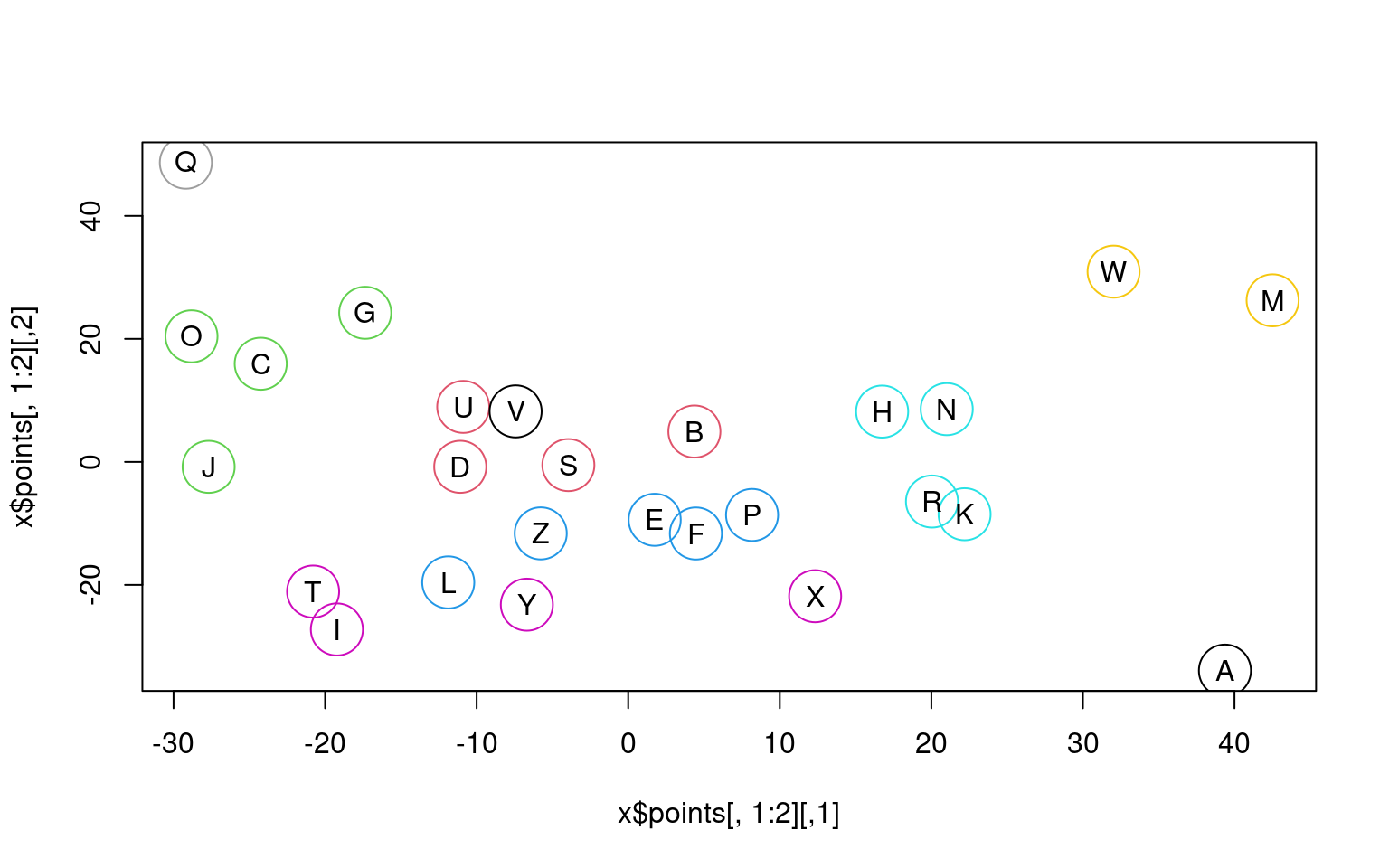
| 2 | 3 | 4 | 5 | 6 | 7 | 8 | 9 | 10 | 11 | 12 | 13 | 14 | 15 | 16 | 17 | 18 | 19 | 20 | 21 | 22 | 23 | 24 | 25 | 26 |
|---|---|---|---|---|---|---|---|---|---|---|---|---|---|---|---|---|---|---|---|---|---|---|---|---|
| 1 | 1 | 1 | 1 | 1 | 1 | 1 | 1 | 1 | 1 | 1 | 1 | 1 | 1 | 1 | 1 | 1 | 1 | 1 | 1 | 1 | 1 | 1 | 1 | 1 |
| 1 | 1 | 1 | 2 | 2 | 2 | 2 | 2 | 2 | 2 | 2 | 2 | 2 | 2 | 2 | 2 | 2 | 2 | 2 | 2 | 2 | 2 | 2 | 2 | 2 |
| 2 | 2 | 2 | 3 | 3 | 3 | 3 | 3 | 3 | 3 | 3 | 3 | 3 | 3 | 3 | 3 | 3 | 3 | 3 | 3 | 3 | 3 | 3 | 3 | 3 |
| 1 | 1 | 1 | 2 | 2 | 2 | 2 | 2 | 2 | 2 | 2 | 2 | 2 | 2 | 2 | 4 | 4 | 4 | 4 | 4 | 4 | 4 | 4 | 4 | 4 |
| 1 | 1 | 1 | 2 | 2 | 2 | 2 | 4 | 4 | 4 | 4 | 4 | 4 | 4 | 4 | 5 | 5 | 5 | 5 | 5 | 5 | 5 | 5 | 5 | 5 |
| 1 | 1 | 1 | 2 | 2 | 2 | 2 | 4 | 4 | 4 | 5 | 5 | 5 | 5 | 5 | 6 | 6 | 6 | 6 | 6 | 6 | 6 | 6 | 6 | 6 |
| 2 | 2 | 2 | 3 | 3 | 3 | 3 | 3 | 3 | 3 | 3 | 3 | 3 | 3 | 3 | 3 | 3 | 3 | 3 | 3 | 3 | 7 | 7 | 7 | 7 |
| 1 | 1 | 1 | 1 | 4 | 4 | 4 | 5 | 5 | 5 | 6 | 6 | 6 | 6 | 6 | 7 | 7 | 7 | 7 | 7 | 7 | 8 | 8 | 8 | 8 |
| 1 | 1 | 3 | 4 | 5 | 5 | 5 | 6 | 6 | 6 | 7 | 7 | 7 | 7 | 7 | 8 | 8 | 8 | 8 | 8 | 8 | 9 | 9 | 9 | 9 |
| 2 | 2 | 2 | 3 | 3 | 3 | 3 | 3 | 3 | 7 | 8 | 8 | 8 | 8 | 8 | 9 | 9 | 9 | 9 | 9 | 9 | 10 | 10 | 10 | 10 |
| 1 | 1 | 1 | 1 | 4 | 4 | 4 | 5 | 5 | 5 | 6 | 6 | 9 | 9 | 9 | 10 | 10 | 10 | 10 | 10 | 10 | 11 | 11 | 11 | 11 |
| 1 | 1 | 1 | 2 | 2 | 2 | 2 | 4 | 4 | 4 | 4 | 9 | 10 | 10 | 10 | 11 | 11 | 11 | 11 | 11 | 11 | 12 | 12 | 12 | 12 |
| 1 | 3 | 4 | 5 | 6 | 6 | 6 | 7 | 7 | 8 | 9 | 10 | 11 | 11 | 11 | 12 | 12 | 12 | 12 | 12 | 12 | 13 | 13 | 13 | 13 |
| 1 | 1 | 1 | 1 | 4 | 4 | 4 | 5 | 5 | 5 | 6 | 6 | 6 | 6 | 6 | 7 | 7 | 7 | 7 | 7 | 7 | 8 | 14 | 14 | 14 |
| 2 | 2 | 2 | 3 | 3 | 3 | 3 | 3 | 3 | 3 | 3 | 3 | 3 | 3 | 12 | 13 | 13 | 13 | 13 | 13 | 13 | 14 | 15 | 15 | 15 |
| 1 | 1 | 1 | 2 | 2 | 2 | 2 | 4 | 4 | 4 | 4 | 4 | 4 | 4 | 4 | 5 | 5 | 5 | 5 | 5 | 5 | 5 | 5 | 5 | 16 |
| 2 | 2 | 2 | 3 | 3 | 3 | 7 | 8 | 8 | 9 | 10 | 11 | 12 | 12 | 13 | 14 | 14 | 14 | 14 | 14 | 14 | 15 | 16 | 16 | 17 |
| 1 | 1 | 1 | 1 | 4 | 4 | 4 | 5 | 5 | 5 | 6 | 6 | 9 | 9 | 9 | 10 | 10 | 10 | 15 | 15 | 15 | 16 | 17 | 17 | 18 |
| 1 | 1 | 1 | 2 | 2 | 2 | 2 | 2 | 2 | 2 | 2 | 2 | 2 | 2 | 2 | 4 | 4 | 4 | 4 | 4 | 4 | 4 | 4 | 18 | 19 |
| 1 | 1 | 3 | 4 | 5 | 5 | 5 | 6 | 6 | 6 | 7 | 7 | 7 | 7 | 7 | 8 | 8 | 15 | 16 | 16 | 16 | 17 | 18 | 19 | 20 |
| 1 | 1 | 1 | 2 | 2 | 2 | 2 | 2 | 2 | 2 | 2 | 2 | 2 | 2 | 2 | 4 | 15 | 16 | 17 | 17 | 17 | 18 | 19 | 20 | 21 |
| 1 | 1 | 3 | 4 | 5 | 7 | 8 | 9 | 9 | 10 | 11 | 12 | 13 | 13 | 14 | 15 | 16 | 17 | 18 | 18 | 18 | 19 | 20 | 21 | 22 |
| 1 | 3 | 4 | 5 | 6 | 6 | 6 | 7 | 7 | 8 | 9 | 10 | 11 | 11 | 11 | 12 | 12 | 12 | 12 | 19 | 19 | 20 | 21 | 22 | 23 |
| 1 | 1 | 3 | 4 | 5 | 5 | 5 | 6 | 10 | 11 | 12 | 13 | 14 | 14 | 15 | 16 | 17 | 18 | 19 | 20 | 20 | 21 | 22 | 23 | 24 |
| 1 | 1 | 3 | 4 | 5 | 5 | 5 | 6 | 10 | 11 | 12 | 13 | 14 | 15 | 16 | 17 | 18 | 19 | 20 | 21 | 21 | 22 | 23 | 24 | 25 |
| 1 | 1 | 1 | 2 | 2 | 2 | 2 | 4 | 4 | 4 | 5 | 5 | 5 | 5 | 5 | 6 | 6 | 6 | 6 | 6 | 22 | 23 | 24 | 25 | 26 |
This seems reasonable, and shows the advantage of the conditional splitting in a hierarchical approach. If we look at the classes matrix, we see the grouping at each level of the clustering, and we can pick out any particular row as a solution.
Model-based clustering for non-gaussian distributions: The flexmix library
Mixtures of gaussians are very widely used, but we sometimes need more flexibility. Just as with regression, sometimes we don’t want to use the guassian error distribution. A good example is for binary data, although likert-scales apply as well. Or consider data where you might have a rank-order constraint. Or if you were to model a pattern of shots on a target or a dartboard, you might model a mixture of a guassians (for the ability of a person) and a low-density uniform (for mistakes that were haphazard), so that you can remove and account for any outliers while still capturing the precision of the person.
The flexmix library provides a set of tools for building
much more general mixture models. There are many built-in options, but
you can also create ‘drivers’ for custom models and mixtures of
models.
A reasonable model for binary behavior such as voting is a binomial model, as it models the probability of agreement directly. Let’s take another look at the Michigan Senate voting data, that we have previously looked at. Can we detect party affiliation by modeling the data as a mixture of binomials?
We could model each person with a single binomial coefficient– each person has a tendency to vote for or against a set of issues, modeled as a probability. But for this case, let’s assume that a “voting bloc” has a tendency to vote similarly, and people belong to a voting block. Then, we can use mixture modeling to identify which voting block they belong to, and what the voting block looks like.
To use flexmix, we need to specify the model we want, which is the FLXMCmbinary. There are dozens of models, including gaussian, and others that we will examine in the next unit.
library(flexmix)

data.raw <- read.csv("misenate.csv")
key <- read.csv("misenate-key.csv", header = F)

keep <- !is.na(rowMeans(data.raw[, -(1:2)]))
data <- data.raw[keep == TRUE, ]
party <- data$Party
votes <- as.matrix(data[, -(1:2)])


## model with a single group is easy;
model1 <- flexmix(votes ~ 1, k = 1, model = FLXMCmvbinary())
model2 <- flexmix(votes ~ 1, k = 2, model = FLXMCmvbinary())

table(party, clusters(model2))
party  1  2
    D  0 44
    R 58  1
party  1  2
    D  0 44
R 58 1 Comp.1 Comp.2
center.Q1 6.379310e-01 0.86666667
center.Q2 2.209931e-165 0.62222222
center.Q3 1.379310e-01 0.73333333
center.Q4 6.724138e-01 0.84444444
center.Q5 3.965517e-01 0.15555556
center.Q6 5.172414e-02 0.33333333
center.Q7 6.896552e-02 1.00000000
center.Q8 3.448276e-02 0.77777778
center.Q9 8.103448e-01 0.93333333
center.Q10 3.448276e-02 0.77777778
center.Q11 2.209931e-165 1.00000000
center.Q12 1.231430e-276 0.15555556
center.Q13 3.448276e-02 0.22222222
center.Q14 6.206897e-01 0.95555556
center.Q15 1.724138e-02 1.00000000
center.Q16 3.448276e-02 1.00000000
center.Q17 5.172414e-02 1.00000000
center.Q18 1.724138e-02 0.91111111
center.Q19 5.172414e-02 0.97777778
center.Q20 2.209931e-165 0.86666667
center.Q21 3.448276e-02 0.91111111
center.Q22 3.897129e-272 0.77777778
center.Q23 1.265983e-252 0.88888889
center.Q24 8.620690e-02 0.91111111
center.Q25 1.724138e-02 0.46666667
center.Q26 8.965517e-01 1.00000000
center.Q27 1.724138e-02 0.82222222
center.Q28 8.793103e-01 0.71111111
center.Q29 1.206897e-01 1.00000000
center.Q30 8.620690e-02 0.73333333
center.Q31 3.506674e-276 0.55555556
center.Q32 5.862069e-01 0.91111111
center.Q33 8.103448e-01 1.00000000
center.Q34 3.448276e-02 0.60000000
center.Q35 8.620690e-01 0.84444444
center.Q36 6.896552e-02 1.00000000
center.Q37 5.172414e-02 0.73333333
[ reached getOption("max.print") -- omitted 17 rows ]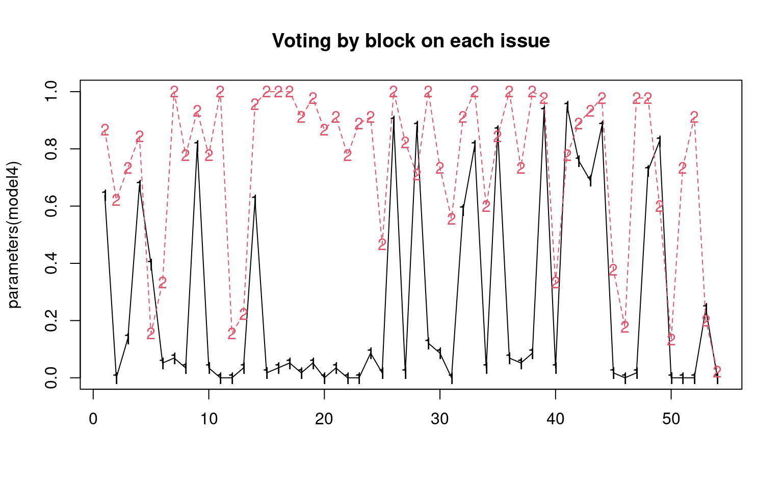
We find that as the number of groups grows, we get different answers different times, and we start losing groups. Also, fitting each model size separately is a bit tedious. Because we can get a solution each time, we’d like to repeat the model from a bunch of different random starting configurations, and just keep the best model we find.
The stepflexmix function takes care of a lot of this for
us. We can specify a range of k values, which tells us the
number of groups to explore. We can also select nrep, which
tells us how many times to fit the model at each level of
k. 20 is fine for exploring, but you may try
nrep values as large as 1000 if you want to be confident
that are getting a consistently good solution.
# set.seed(100)

modelsx <- stepFlexmix(votes ~ 1, k = 1:6, model = FLXMCmvbinary(), nrep = 10, drop = FALSE)
1 : * * * * * * * * * *
2 : * * * * * * * * * *
3 : * * * * * * * * * *
4 : * * * * * * * * * *
5 : * * * * * * * * * *
6 : * * * * * * * * * *
Call:
stepFlexmix(votes ~ 1, model = FLXMCmvbinary(), k = 1:6, nrep = 10,
    drop = FALSE)

  iter converged k k0    logLik      AIC      BIC      ICL
1    2      TRUE 1  1 -2994.339 6096.677 6238.952 6238.952
2    5      TRUE 2  2 -1697.609 3613.218 3900.404 3900.404
3   13      TRUE 3  3 -1586.562 3501.123 3933.219 3933.446
4   24      TRUE 4  4 -1531.377 3500.754 4077.759 4078.934
5   27      TRUE 4  5 -1495.364 3428.728 4005.734 4006.215
6    9      TRUE 5  6 -1483.637 3515.273 4237.189 4237.564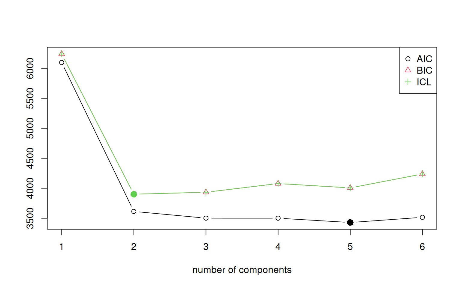
Unlike the mclust library, flexmix plots
BIC so that lower is better. Here, the BIC tends to favor two groups,
but the AIC favors 5 or more groups. Notice that drop, which defaults to
TRUE, can prevent groups from being completely dropped. If we look at
the output, we se that even for this case, the ultimate value of k that
was achieved is often not the same as the starting value (k0), and we
never ended up with more than 6 groups. Notice also that the best
solutions have slightly different BIC values–even within 6-group
solutions. This means that we would probably want to increase nrep to
make sure we consistently find the best group.
A number of functions let us extract the model and extract
information from them model. We can extract the best model using
getModel; if we specify the statistic (“BIC” or “AIC”) it
will pick out that model; if we specify a number, it will pick out the
model with that number of components.
Call:
stepFlexmix(votes ~ 1, model = FLXMCmvbinary(), k = 2, nrep = 10,
    drop = FALSE)

Cluster sizes:
 1  2
58 45

convergence after 5 iterations
Call:
stepFlexmix(votes ~ 1, model = FLXMCmvbinary(), k = 2, nrep = 10,
    drop = FALSE)

       prior size post>0 ratio
Comp.1 0.563   58     58     1
Comp.2 0.437   45     45     1

'log Lik.' -1697.609 (df=109)
AIC: 3613.218 BIC: 3900.404 Comp.1 Comp.2 Comp.3 Comp.4
center.Q1 6.590821e-01 5.385580e-01 7.914564e-01 0.92547077
center.Q2 0.000000e+00 0.000000e+00 4.173555e-01 0.74564535
center.Q3 1.363851e-01 1.537639e-01 4.786232e-01 0.88828708
center.Q4 8.633822e-01 7.821707e-02 7.394393e-01 0.88810414
center.Q5 2.949596e-01 7.706432e-01 1.042248e-01 0.18649297
center.Q6 6.819295e-02 1.467817e-180 5.224036e-02 0.52208982
center.Q7 6.819295e-02 0.000000e+00 1.000000e+00 1.00000000
center.Q8 4.546196e-02 0.000000e+00 4.267670e-01 1.00000000
center.Q9 9.545387e-01 3.849528e-01 8.957758e-01 0.92540262
center.Q10 4.546196e-02 0.000000e+00 4.267670e-01 1.00000000
center.Q11 0.000000e+00 0.000000e+00 9.478879e-01 1.00000000
center.Q12 0.000000e+00 0.000000e+00 5.211526e-02 0.22378986
center.Q13 2.251728e-02 7.760340e-02 1.613233e-01 0.25752138
center.Q14 7.728181e-01 7.699984e-02 8.957758e-01 1.00000000
center.Q15 0.000000e+00 0.000000e+00 1.000000e+00 1.00000000
center.Q16 0.000000e+00 7.688061e-02 1.000000e+00 1.00000000
center.Q17 4.546196e-02 5.440720e-88 1.000000e+00 1.00000000
center.Q18 2.273098e-02 0.000000e+00 7.394396e-01 1.00000000
[ reached getOption("max.print") -- omitted 36 rows ]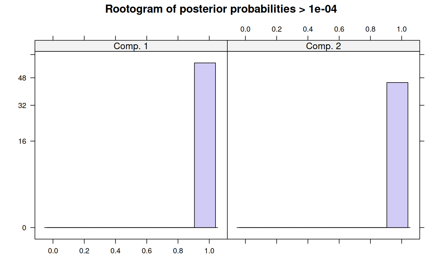
                  Comp.1     Comp.2
center.Q1   6.379310e-01 0.86666667
center.Q2   3.377767e-88 0.62222222
center.Q3   1.379310e-01 0.73333333
center.Q4   6.724138e-01 0.84444444
center.Q5   3.965517e-01 0.15555556
center.Q6   5.172414e-02 0.33333333
center.Q7   6.896552e-02 1.00000000
center.Q8   3.448276e-02 0.77777778
center.Q9   8.103448e-01 0.93333333
center.Q10  3.448276e-02 0.77777778
center.Q11  3.377767e-88 1.00000000
center.Q12 2.313951e-133 0.15555556
center.Q13  3.448276e-02 0.22222222
center.Q14  6.206897e-01 0.95555556
center.Q15  1.724138e-02 1.00000000
center.Q16  3.448276e-02 1.00000000
center.Q17  5.172414e-02 1.00000000
center.Q18  1.724138e-02 0.91111111
center.Q19  5.172414e-02 0.97777778
center.Q20  3.377767e-88 0.86666667
center.Q21  3.448276e-02 0.91111111
center.Q22 2.314036e-133 0.77777778
center.Q23 8.091148e-126 0.88888889
center.Q24  8.620690e-02 0.91111111
center.Q25  1.724138e-02 0.46666667
center.Q26  8.965517e-01 1.00000000
center.Q27  1.724138e-02 0.82222222
center.Q28  8.793103e-01 0.71111111
center.Q29  1.206897e-01 1.00000000
center.Q30  8.620690e-02 0.73333333
center.Q31 1.483196e-142 0.55555556
center.Q32  5.862069e-01 0.91111111
center.Q33  8.103448e-01 1.00000000
center.Q34  3.448276e-02 0.60000000
center.Q35  8.620690e-01 0.84444444
center.Q36  6.896552e-02 1.00000000
center.Q37  5.172414e-02 0.73333333
[ reached getOption("max.print") -- omitted 17 rows ] [1] 1 1 1 1 1 1 1 1 1 1 1 1 1 1 1 1 1 1 1 1 1 1 1 1 1 1 1 1 1 1 1 1 1 1 1 1 1 1
[39] 1 1 1 1 1 1 1 1 1 1 1 1 1 1 1 1 1 1 1 1 2 2 2 2 2 2 2 2 2 2 2 2 2 2 2 2 2
[ reached getOption("max.print") -- omitted 28 entries ]
party  1  2
    D  0 44
    R 58  1
If you plot a model, it shows a ‘rootogram’. This is a histogram of the likelihood of each item being in each model. Ideally, if you have clear separation, you have a lot of densiity at the edges, without many ambiguous cases in the middle.
We can pick out an arbitrary model too:
Call:
stepFlexmix(votes ~ 1, model = FLXMCmvbinary(), k = 4, nrep = 10,
    drop = FALSE)

Cluster sizes:
 1  2  3  4
16 25 19 43

convergence after 24 iterations
Call:
stepFlexmix(votes ~ 1, model = FLXMCmvbinary(), k = 4, nrep = 10,
    drop = FALSE)

       prior size post>0 ratio
Comp.1 0.154   16     24 0.667
Comp.2 0.239   25     25 1.000
Comp.3 0.188   19     29 0.655
Comp.4 0.419   43     47 0.915

'log Lik.' -1531.377 (df=219)
AIC: 3500.754 BIC: 4077.759 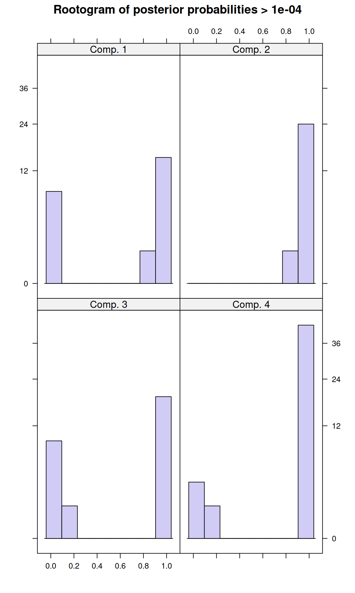
                  Comp.1     Comp.2       Comp.3       Comp.4
center.Q1   5.582242e-01 0.92005437 7.917557e-01 6.755954e-01
center.Q2   0.000000e+00 0.80769584 4.180739e-01 0.000000e+00
center.Q3   1.892895e-01 0.87985283 5.845580e-01 1.158723e-01
center.Q4   6.341160e-02 0.87830407 8.449486e-01 8.804982e-01
center.Q5   7.585575e-01 0.20282557 5.168629e-02 2.775830e-01
center.Q6   1.938807e-65 0.56622475 5.384051e-02 6.952210e-02
center.Q7   1.892953e-01 1.00000000 1.000000e+00 4.634806e-02
center.Q8   6.309844e-02 1.00000000 4.831653e-01 4.634806e-02
center.Q9   4.321245e-01 0.91886889 9.483165e-01 9.536481e-01
center.Q10  6.309844e-02 1.00000000 5.348487e-01 2.317403e-02
center.Q11  6.309844e-02 1.00000000 1.000000e+00 0.000000e+00
center.Q12  6.309844e-02 0.24339333 5.686146e-72 0.000000e+00
center.Q13  6.325828e-02 0.24220711 2.082452e-01 2.311533e-02
center.Q14  1.894082e-01 1.00000000 8.966331e-01 7.878756e-01
center.Q15  1.261969e-01 1.00000000 1.000000e+00 0.000000e+00
center.Q16  1.892953e-01 1.00000000 1.000000e+00 0.000000e+00
center.Q17  1.263650e-01 1.00000000 1.000000e+00 4.628633e-02
center.Q18  6.309844e-02 1.00000000 7.932661e-01 2.317403e-02
[ reached getOption("max.print") -- omitted 36 rows ] [1] 1 1 1 1 1 1 1 1 4 1 4 1 1 4 4 1 4 4 4 4 1 4 4 4 4 4 4 4 4 4 4 4 4 4 4 4 4 4
[39] 4 4 4 4 4 4 4 4 4 4 4 4 4 4 4 4 4 4 1 1 1 3 3 3 3 3 3 3 3 3 3 3 3 3 3 3 3
[ reached getOption("max.print") -- omitted 28 entries ]
party  1  2  3  4
    D  1 25 18  0
R 15 0 1 43matplot(parameters(bestmodel), 1:54, type = "o", ylab = "Issue", xlab = "Model parameter value")
grid()
If forced to classify the politicians into 4 parties, we usually get two democrats and two republicans, but sometimes one of the groups is a bit mixed. We could maybe sort the issues (since they are arbitrary) to get a better picture. We can make a table with declared party membership to determine who belongs in which group. Then, we can arrange issues using another clustering solution. In fact, let’s mix a simple k-means clustering on the answers to find an ordering of questions for which issues are grouped together based on how different groups vote.
# set.seed(101)
tab <- table(party, clusters(bestmodel))
gparty <- c("D", "R")[apply(tab, 2, which.max)]
p <- parameters(bestmodel)

grp <- kmeans(p, centers = 7)
## find the mean positive vote probability across cluster. grpord <-
## rank(aggregate(rowMeans(p),list(grp$cluster),mean)$x)

ord <- order(grp$cluster)  #(grpord[grp$cluster])
par(mar = c(3, 25, 2, 1), las = 1)
matplot(p[ord, ], 1:54, pch = gparty, type = "o", yaxt = "n", ylab = "", xlab = "Agreement with rater on bill")
grid()
axis(2, 1:54, paste(paste(key$V1, key$V2)[ord], sort(grp$cluster)), cex.axis = 0.75)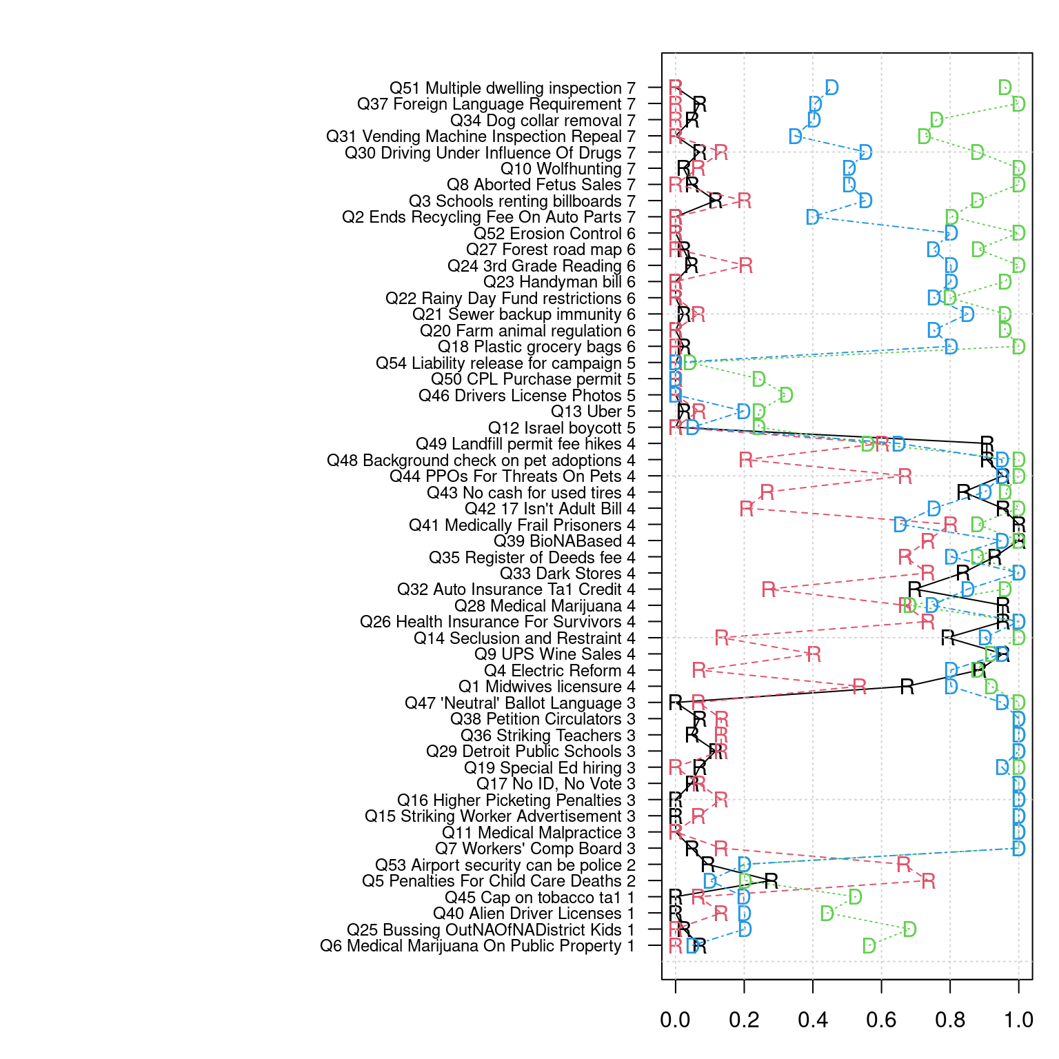
This clustered questions into 7 groups, then just displayed them in order of the (arbitrary) group number. Looking at the bills, it is difficult to determine why they clustered together, or why the 4-party solution divided parties on specific issues, but someone who follows Michigan politics may learn important things from this solution.
FMM vs K-means
These two approaches are often similar, but the model-based assumptions can enable some interesting applications. Suppose you have two groups with the SAME means, but different variance. E.g., expert marksmen and novices.
data2 <- matrix(c(rnorm(200, mean = centers[, 1], sd = 0.1), rnorm(200, mean = centers[,
    2], sd = 1)), ncol = 2, byrow = T)

colnames(data2) <- c("V1", "V2")
plot(data2, col = rep(c("red", "darkgreen"), each = 100))
points(t(centers), pch = 16, cex = 2, col = c("red", "darkgreen"))
A normal k-means would probably find one group. But because the distributions violate the shape of the normal, we might be able to separate them better.
----------------------------------------------------
Gaussian finite mixture model fitted by EM algorithm
----------------------------------------------------

Mclust VII (spherical, varying volume) model with 2 components:

 log-likelihood   n df       BIC      ICL
      -224.8852 200  7 -486.8586 -498.001

Clustering table:
  1   2
105 95 
     1  2
  1 99  1
  2  6 94
This actually does very well at classifying the two groups as two overlapping normal distributions with different variances.

      1   2
  1   0 100
  2  37  63
The kmeans completely fails at this, as expected. But if we constrain the mclust so that the distributions have to be the same size, they are unlikely to overlap, and we might see the same thing:

We can see from the BIC plot that there are a handful of models that peak at 2 components, and then a bunch of others that grow slowly. The lower set of models mostly appear to have “E” as their first character, which indicates equal-volume clusters. EII is maybe the simplest of these (equal volume spherical), but if we allow it any of three of these, it finds EVE with 7 clusters is best–these take on different shapes and orientations.
modelEEE <- Mclust(data2, modelNames = c("EEE", "EII", "EVE"))
plot(modelEEE, what = "classification")
The first E stands for equal volume/size, and the best model has a single center cluster orbitted by other clusters.
Other libraries
In their paper on mclust, (https://journal.r-project.org/archive/2016/RJ-2016-021/RJ-2016-021.pdf), Scrucca et al. (2016) showed that mclust and flexmix are the two most popular libraries for mixture modeling in R. Aside from mclust and flexmix, there are a number of libraries in R that support mixture models:
- bgmm: Gaussian and ‘belief’-based mixture modeling, for ‘partially-supervised’ clustering. If classification is fully-supervised, and clustering is unsupervised, partially-supervised fits in the middle, where the clustering is still driven by the observed features, but informed by probabilistic or fuzzy assessments of labels we are trying to predict.
- EMCluster: An efficient algorithm for finite gaussian mixtures and semi-supervised classification.
- mixtools: mixture modeling allowing several distributions, mixtures of regressions, mixtures of experts.
- mixture: implements 14 mixture models with different distributions for model-based clustering and classification. It appears to overlap with the different models mclust provides
- Rmixmod: an R interface to MIXMOD, for supervised, unsupervised, and semi-supervised classification and clustering using mixture modeling. The base software is in C++ and has available interfaces in python as well.
As you can see, this is an exciting area with a lot of cutting-edge research.