Mixture Modeling: Mixture of Regressions

Mixture Modeling: Mixtures of regressions.

A mixture model is a probabilistic model for representing the presence of sub-populations within an overall population, without requiring that an observed data-set should identify the sub-population to which an individual observation belongs. We previously used a very simple model–where each variable is defined by its mean and standard deviation, to do model-based clustering. But mixture modeling permits finding mixtures of hidden group memberships for other kinds of models, including regression models. This sometimes enables you to identify sets of distinct relationships amongst sub-groups, hidden within a larger population. The goal of mixture modeling is to model your data as a mixture of processes or populations that have distinct patterns of data.

Example 1: Two linear models

Suppose we have two types of people: those who like romantic comedy movies, and those who hate romantic comedies. On a movie rating site, we have measured ratings of anonymous people rating how much they like movies, that we have already measured on how romantic they are. Thus, we’d expect a crossing pattern in the data, like we see below. If we knew why type of person each person was, we’d be able to fit separate regression models, but we don’t.

set.seed(100)
x1 <- rnorm(1000) * 50
x2 <- rnorm(1000) * 50
y1 <- x1 * 3 + 10 + rnorm(1000) * 30
y2 <- -3 * x2 + 25 + rnorm(1000) * 50
x <- c(x1, x2)
y <- c(y1, y2)
par(mfrow = c(1, 3))
plot(x1, y1)
plot(x2, y2)
plot(x, y)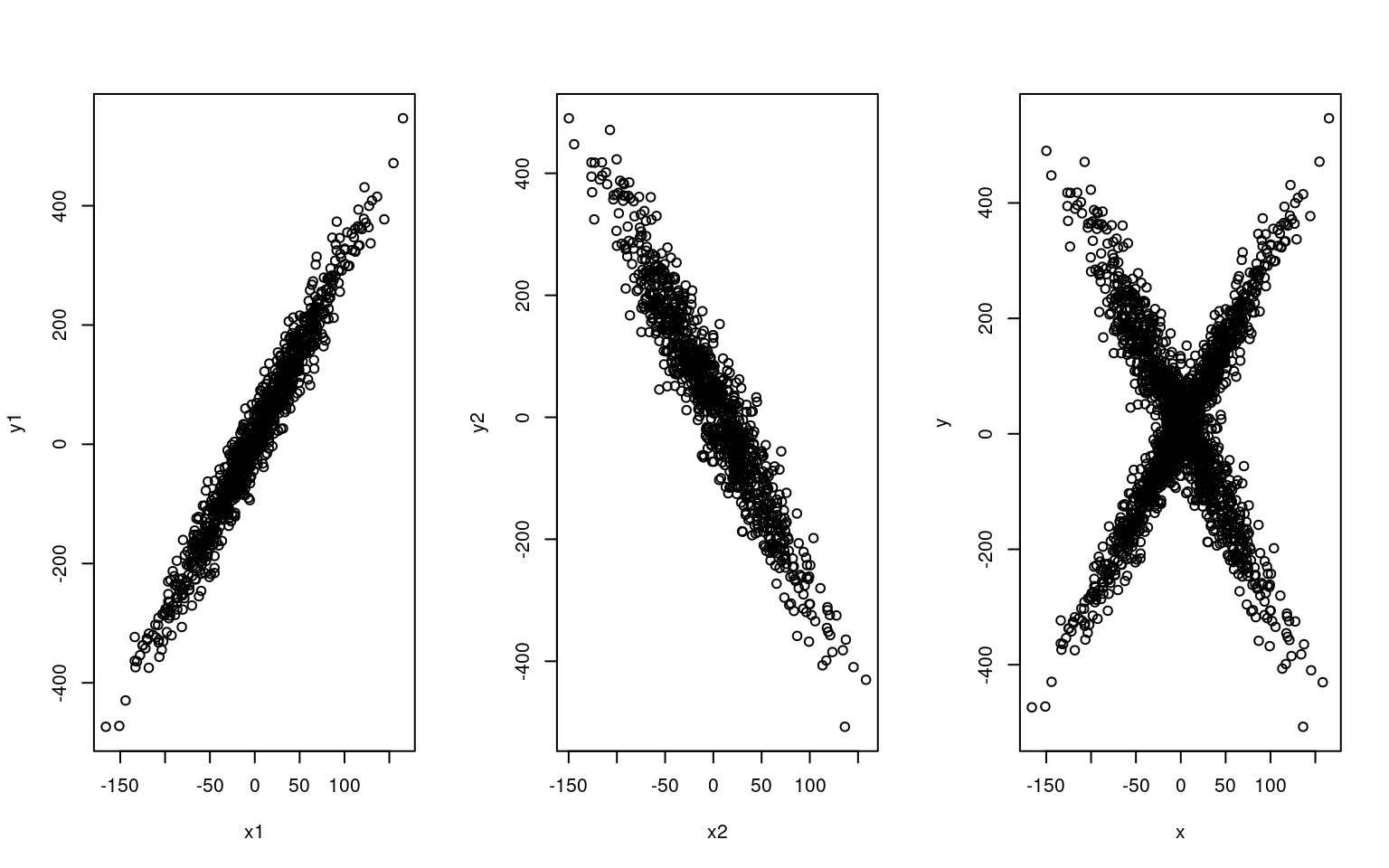

lm(y1 ~ x1)


Call:
lm(formula = y1 ~ x1)

Coefficients:
(Intercept)           x1  
      9.573        2.976

lm(y2 ~ x2)


Call:
lm(formula = y2 ~ x2)

Coefficients:
(Intercept)           x2  
     25.196       -3.097

If we try to fit data by using a single linear regression, we fail:

plot(x, y)
lm1 <- lm(y ~ x)
summary(lm1)


Call:
lm(formula = y ~ x)

Residuals:
    Min      1Q  Median      3Q     Max 
-537.79 -102.55    1.96  102.96  513.75 

Coefficients:
            Estimate Std. Error t value Pr(>|t|)    
(Intercept) 18.26748    3.53271   5.171 2.56e-07 ***
x            0.08846    0.07026   1.259    0.208    
---
Signif. codes:  0 '***' 0.001 '**' 0.01 '*' 0.05 '.' 0.1 ' ' 1

Residual standard error: 158 on 1998 degrees of freedom
Multiple R-squared:  0.0007929, Adjusted R-squared:  0.0002928 
F-statistic: 1.586 on 1 and 1998 DF,  p-value: 0.2081

abline(lm1$coefficients, col = "gold", lwd = 3)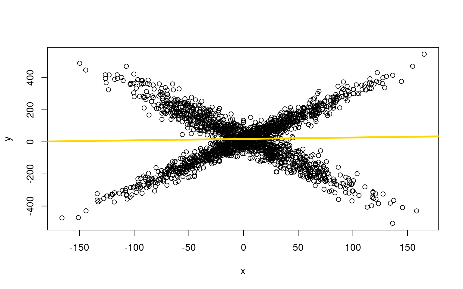

And from summary(lm1), R-squared = 0.0008135

summary(lm1)


Call:
lm(formula = y ~ x)

Residuals:
    Min      1Q  Median      3Q     Max 
-537.79 -102.55    1.96  102.96  513.75 

Coefficients:
            Estimate Std. Error t value Pr(>|t|)    
(Intercept) 18.26748    3.53271   5.171 2.56e-07 ***
x            0.08846    0.07026   1.259    0.208    
---
Signif. codes:  0 '***' 0.001 '**' 0.01 '*' 0.05 '.' 0.1 ' ' 1

Residual standard error: 158 on 1998 degrees of freedom
Multiple R-squared:  0.0007929, Adjusted R-squared:  0.0002928 
F-statistic: 1.586 on 1 and 1998 DF,  p-value: 0.2081

In the example above, it is quite obvious we are missing something. But if we had more noise, or many variables, we might not notice this pattern, and just determine that there was no predictability on average. But there is a very systematic pattern within the data we might be able to uncover–if only we knew which group people were in. But this problem is just like model-based clustering. What if we could both fit two separate models and determine which group each person belongs to? We can do that using the flexmix library.

Fitting mixtures of regressions using E-M and flexmix

If we could use the same approach as with clustering, but instead of gaussians around means, we might have each sub-group defined by a linear model. In this case, as long as we can produce a likelihood estimate for a model, we can use the E-M algorithm to identify and estimate the groups. That is, we can fit a model to a subgroup, obtain the maximum likelihood estimate, then place each observation in the model it is best described by, and repeat until things settle down.

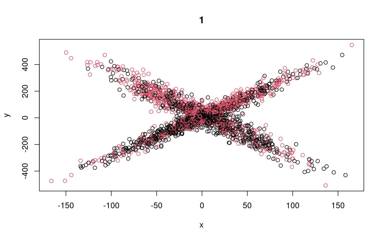
To review: E-M stands for Expectation-Maximization. It is an iterative process whereby you apply two complementary processes. Suppose you assume there are two sub-groups. First, randomly assign members to either of the sub-groups. Next, you compute a maximum likelihood (ML) estimate for each sub-group. Now, because of random variation, there are likely to be members of one group that are better described by the other group (in terms of likelihood). You then apply the ‘maximization’ step to re-sort data into the group that better describes them. You repeat this process, re-estimating your models and re-sorting members until nobody is better described by a model that they are not in. Original research on the E-M algorithm proved that it would converge to a local maximum; you might not get the global maximum however, so you typically repeat the process many times and pick the best outcome you find.

This is possible to do by hand, and in this case is not too complicated.

split <- rep(1:2, 1000)

plot(x, y, col = split)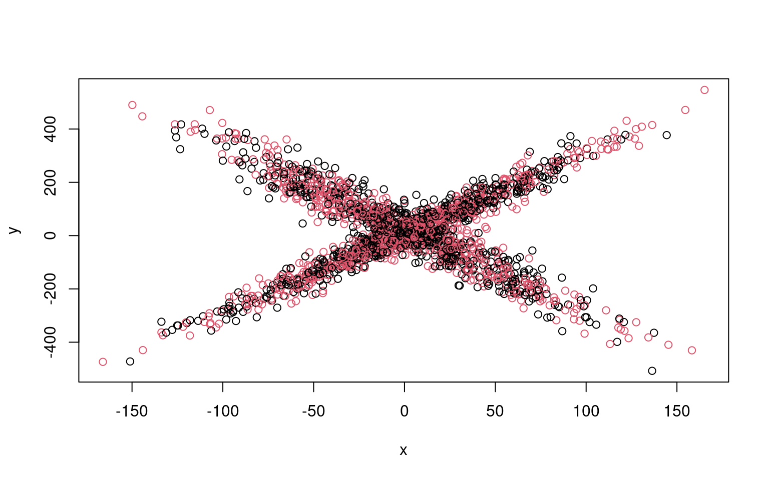

for (i in 1:5) {

    lm1 <- glm(y[split == 1] ~ x[split == 1])
    lm2 <- glm(y[split == 2] ~ x[split == 2])

    ## Compute residuals of all the data for the two models
    res1 <- (predict(lm1, data.frame(x)) - y)
    res2 <- (predict(lm2, data.frame(x)) - y)

    likelihood <- cbind(dnorm(res1, mean = 0, sd = sd(res1)), dnorm(res2, mean = 0,
        sd = sd(res2)))

    split <- apply(likelihood, 1, which.max)
    plot(x, y, col = split, main = i)
    print(lm1)
    print(lm2)

}


Call:  glm(formula = y[split == 1] ~ x[split == 1])

Coefficients:
  (Intercept)  x[split == 1]  
     17.09494        0.08062  

Degrees of Freedom: 999 Total (i.e. Null);  998 Residual
Null Deviance:      23240000 
Residual Deviance: 23220000     AIC: 12900

Call:  glm(formula = y[split == 2] ~ x[split == 2])

Coefficients:
  (Intercept)  x[split == 2]  
     19.43532        0.09495  

Degrees of Freedom: 999 Total (i.e. Null);  998 Residual
Null Deviance:      26660000 
Residual Deviance: 26640000     AIC: 13030


Call:  glm(formula = y[split == 1] ~ x[split == 1])

Coefficients:
  (Intercept)  x[split == 1]  
     -14.6458         0.2283  

Degrees of Freedom: 1058 Total (i.e. Null);  1057 Residual
Null Deviance:      23420000 
Residual Deviance: 23290000     AIC: 13600

Call:  glm(formula = y[split == 2] ~ x[split == 2])

Coefficients:
  (Intercept)  x[split == 2]  
     54.99022       -0.01926  

Degrees of Freedom: 940 Total (i.e. Null);  939 Residual
Null Deviance:      24090000 
Residual Deviance: 24090000     AIC: 12230


Call:  glm(formula = y[split == 1] ~ x[split == 1])

Coefficients:
  (Intercept)  x[split == 1]  
    -107.3808         0.1218  

Degrees of Freedom: 997 Total (i.e. Null);  996 Residual
Null Deviance:      9401000 
Residual Deviance: 9364000  AIC: 11970

Call:  glm(formula = y[split == 2] ~ x[split == 2])

Coefficients:
  (Intercept)  x[split == 2]  
    143.75711       -0.07905  

Degrees of Freedom: 1001 Total (i.e. Null);  1000 Residual
Null Deviance:      8980000 
Residual Deviance: 8964000  AIC: 11970


Call:  glm(formula = y[split == 1] ~ x[split == 1])

Coefficients:
  (Intercept)  x[split == 1]  
    -109.0668         0.1154  

Degrees of Freedom: 984 Total (i.e. Null);  983 Residual
Null Deviance:      9183000 
Residual Deviance: 9150000  AIC: 11800

Call:  glm(formula = y[split == 2] ~ x[split == 2])

Coefficients:
  (Intercept)  x[split == 2]  
    142.20347       -0.08373  

Degrees of Freedom: 1014 Total (i.e. Null);  1013 Residual
Null Deviance:      9173000 
Residual Deviance: 9155000  AIC: 12130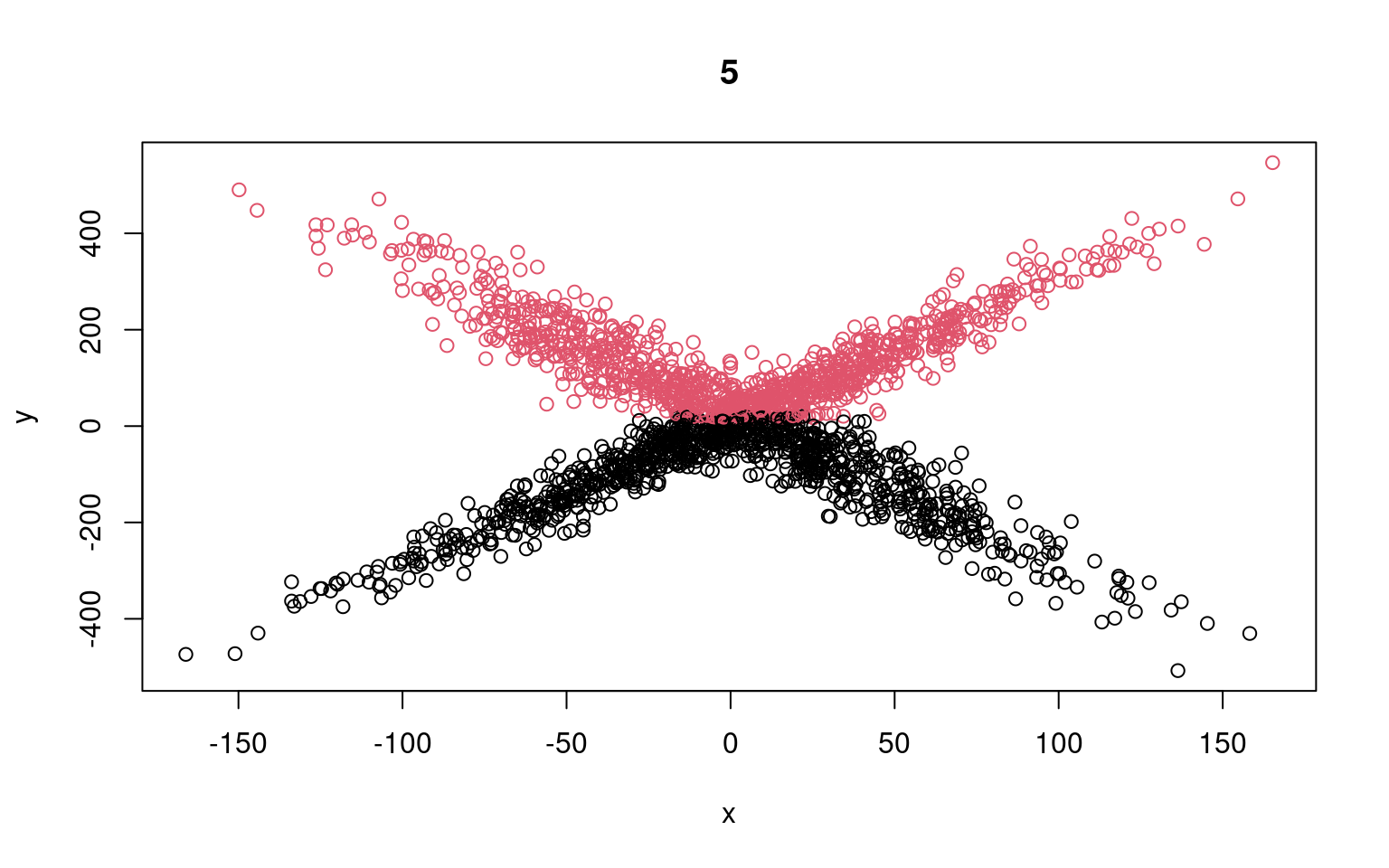


Call:  glm(formula = y[split == 1] ~ x[split == 1])

Coefficients:
  (Intercept)  x[split == 1]  
     -110.747          0.109  

Degrees of Freedom: 971 Total (i.e. Null);  970 Residual
Null Deviance:      8973000 
Residual Deviance: 8944000  AIC: 11640

Call:  glm(formula = y[split == 2] ~ x[split == 2])

Coefficients:
  (Intercept)  x[split == 2]  
    140.63808       -0.08789  

Degrees of Freedom: 1027 Total (i.e. Null);  1026 Residual
Null Deviance:      9374000 
Residual Deviance: 9354000  AIC: 12290

We can see that the two models typically found have low slope, and a difference in the intercept. But the two models are not that great; if we happened upon a pair of models that crossed, the solution would be better. We might have to run a few dozen or hundreds of times to find that one. The flexmix library automates this all for us.

Flexmix modeling:

The ‘flexmix’ package allows us to do this very easily. FlexMix implements a general framework for fitting discrete mixtures of regression models in the R statistical computing environment.

library(flexmix)
model <- flexmix(y ~ x, k = 2)
plot(x, y, col = clusters(model))
abline(parameters(model)[1:2, 1], col = "blue", lwd = 3)
abline(parameters(model)[1:2, 2], col = "green", lwd = 3)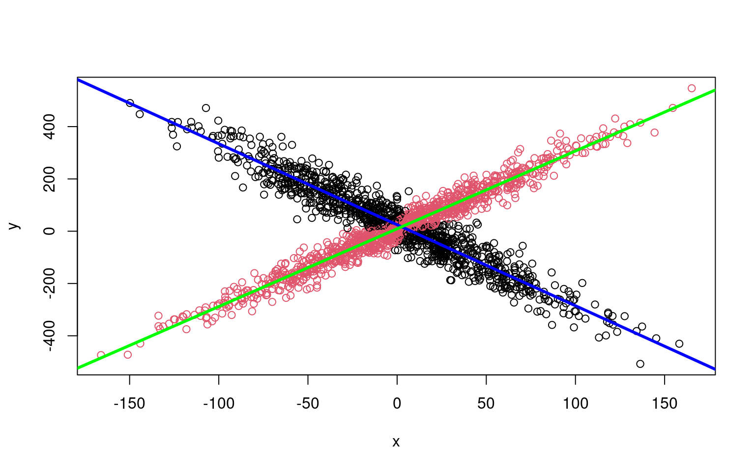

Along with being easier to use, it gets the original (crossing) model right almost every time–there are other heuristics used for model search that help the flexmix model get a better solution than we get when building by hand.

The summary() method gives the estimated prior probabilities, the number of observations assigned to the corresponding clusters, the number of observations where posterior probability > \(\delta\) for each component (with a default of .0001). This indicates the proportion and number of observations that are fit even a little bit by the model, in comparison to those fit best by the model. In the above example, one component has a ratio of around .78–there were 1375 points that had non-zero likelihood of being in that group, and of those 78% were best fit by that group. The distribution of those likelihoods is shown as a rootogram (with the count scale is transformed). Histograms or rootograms of the posterior class probabilities can be used to visually assess the cluster structure. Rootograms are very similar to histograms, the only difference is that the height of the bars correspond to square roots of counts rather than the counts themselves, so that low counts are more visible and peaks less so.

summary(model)


Call:
flexmix(formula = y ~ x, k = 2)

       prior size post>0 ratio
Comp.1 0.494  933   1501 0.622
Comp.2 0.506 1067   1375 0.776

'log Lik.' -11251.22 (df=7)
AIC: 22516.45   BIC: 22555.66

plot(model)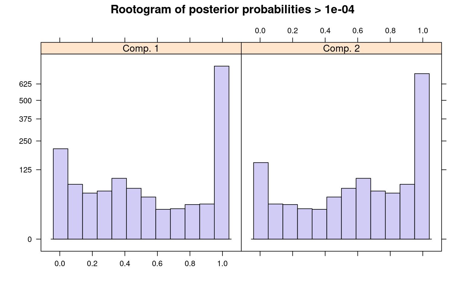

parameters(model)

                    Comp.1    Comp.2
coef.(Intercept) 24.607277  9.317427
coef.x           -3.098094  2.974661
sigma            47.842963 31.950443

When interpreting rootograms, keep in mind that there is no ‘ground truth’. A peak near probability 1 indicates that many of the points are overwhelmingly well-represented by that cluster. A peak near 0 would indicate that many points clearly don’t fit the category (which is also usually good). Points in the middle indicate a lack of separation–there are points that are only moderately well-described by that group, which should be considered with respect to the number of groups you think exist.

Example: A mixture of variances

Mixture modeling can be used to identify outliers or select elements that are caused by the same process but have mutch larger variance. Sometimes, skewed distributions with long tails are modeled as mixtures of two gaussians–one to capture the fairly symmetrical centroid of the distribution, and a second to capture the long tail. At the end of the day, you may treat the tail as a nuisance and use the centroid model as the one you care about.

Random 1000 variables for x and y

x1 <- rep(1:10, 50)
x2 <- rep(1:10, each = 5)
y1 <- 3 * x1 + 10 + rnorm(500) * 3
y2 <- 3 * x2 + 10 + rnorm(50) * 50
x <- c(x1, x2)
y <- c(y1, y2)
plot(x, y)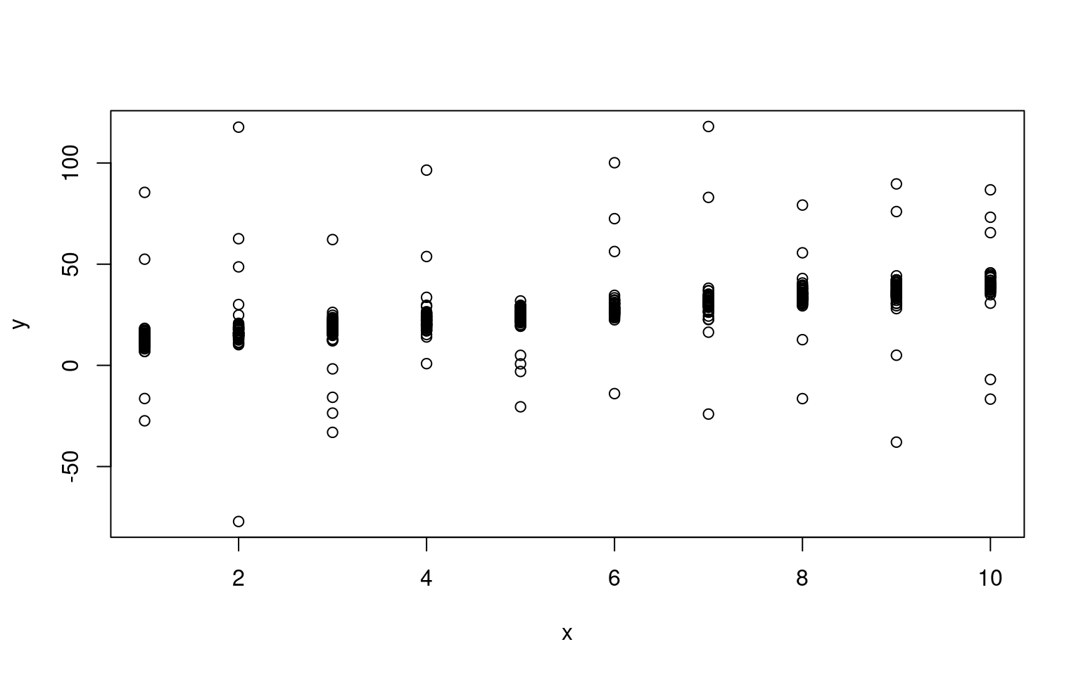

Notice that we have a clear linear relationship, along with a handful of outliers. For a regular maxmimum-likelihood model, these outliers present a problem because they are either very unlikely (punishing the model), or the model’s variance must get larger to make them reasonable, making all the other data less likely.

library(flexmix)
model2a <- flexmix(y ~ x, k = 1)
summary(model2a)


Call:
flexmix(formula = y ~ x, k = 1)

       prior size post>0 ratio
Comp.1     1  550    550     1

'log Lik.' -2222.624 (df=3)
AIC: 4451.247   BIC: 4464.177

model2b <- flexmix(y ~ x, k = 2)
summary(model2b)


Call:
flexmix(formula = y ~ x, k = 2)

        prior size post>0  ratio
Comp.1 0.9025  505    510 0.9902
Comp.2 0.0975   45    550 0.0818

'log Lik.' -1639.939 (df=7)
AIC: 3293.878   BIC: 3324.048

parameters(model2b)

                   Comp.1    Comp.2
coef.(Intercept) 9.984226 16.913096
coef.x           3.015274  2.298855
sigma            2.873646 43.135081

clusters(model2b)

 [1] 1 1 1 1 1 1 1 1 1 1 1 1 1 1 1 1 1 1 1 1 1 1 1 1 1 1 1 1 1 1 1 1 1 1 1 1 1 1
[39] 1 1 1 1 1 1 1 1 1 1 1 1 1 1 1 1 1 1 1 1 1 1 1 1 1 1 1 1 1 1 1 1 1 1 1 1 1
 [ reached getOption("max.print") -- omitted 475 entries ]

In this case, the 2-group model will often select 40/50 of the outliers to be in the secondary group. We’d like to know whether the 2-group solution is any better? We can use a criterion such as BIC to do this.

Bayesian Information Criterion (BIC)

The BIC is a statistic that is based on both the likelihood of the data AND a punishing factor related to the number of parameters used. If you have three parameters for a default model (intercept, slope, and variance), you would have six for a model with two clusters, and nine for one with three. To use the BIC statistic, you can just compare across models and determine which is the smallest. This model provides the best trade-off between accuracy and complexity. However, sometimes the differences are small and you still may prefer a more complex model for other reasons.

In the above example, the BIC is given as part of the output of each model, or we can get it directly:

BIC(model2a)

[1] 4464.177

BIC(model2b)

[1] 3324.048

Here, model2b has a much smaller BIC, so we would prefer this one–the two-group model. We’d like to be able to automate this, looking across a number of options; we’d also like to run this many times (and with more than just 2 groups) and see if there are any better solutions. Here is a way to do both. In the stepFlexmix function, it allows you to specify the numbers of clusters to test, and the number of repetitions at each configuration. We can then select the one with the smallest BIC using the getModel() function

models <- stepFlexmix(y ~ x, k = 1:5, nrep = 10)

1 : * * * * * * * * * *
2 : * * * * * * * * * *
3 : * * * * * * * * * *
4 : * * * * * * * * * *
5 : * * * * * * * * * *

models


Call:
stepFlexmix(y ~ x, k = 1:5, nrep = 10)

  iter converged k k0    logLik      AIC      BIC      ICL
1    2      TRUE 1  1 -2222.624 4451.247 4464.177 4464.177
2    9      TRUE 2  2 -1639.939 3293.877 3324.047 3346.978
3  200     FALSE 3  3 -1636.294 3294.589 3341.998 3644.351
4  200     FALSE 4  4 -1635.600 3301.200 3365.849 3840.103
5  200     FALSE 5  5 -1635.334 3308.668 3390.556 4024.163

summary(models)

     Length       Class        Mode 
          1 stepFlexmix          S4

plot(models)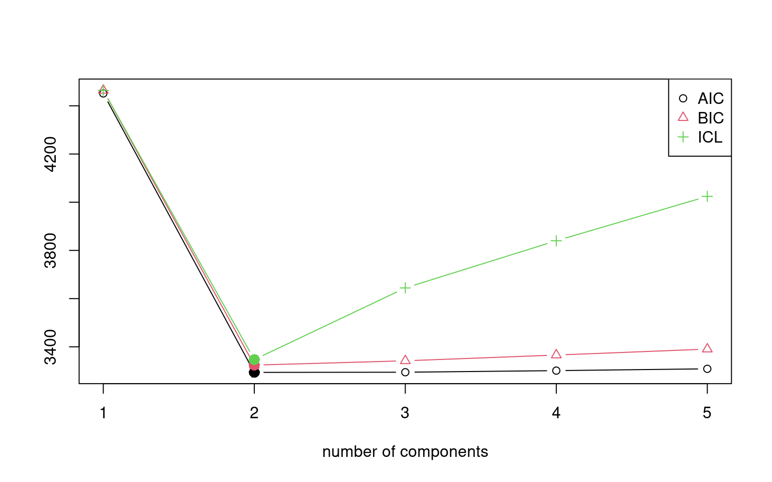

model <- getModel(models, "BIC")
model


Call:
stepFlexmix(y ~ x, k = 2, nrep = 10)

Cluster sizes:
  1   2 
505  45 

convergence after 9 iterations

plot(model)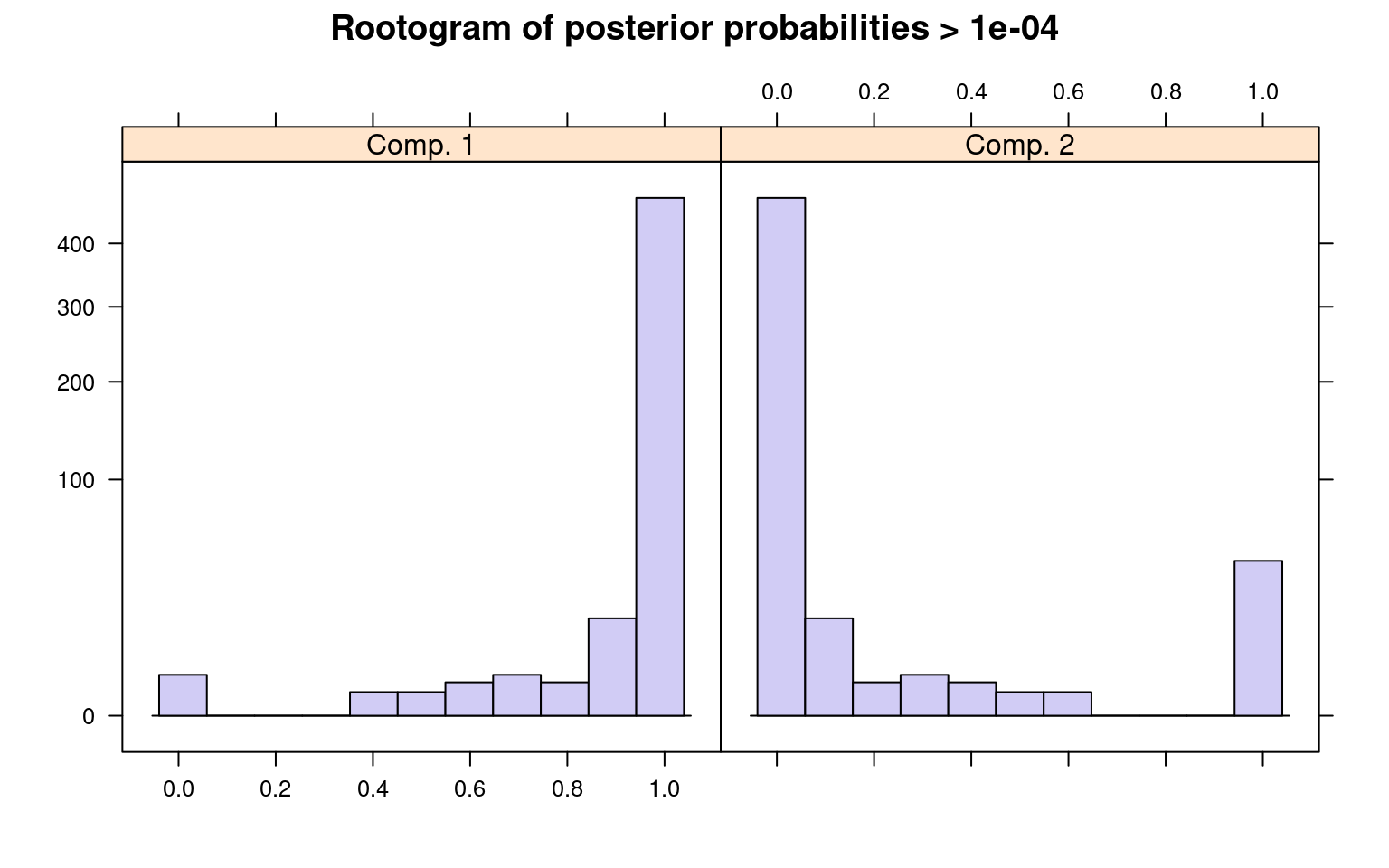

summary(model)


Call:
stepFlexmix(y ~ x, k = 2, nrep = 10)

        prior size post>0  ratio
Comp.1 0.9024  505    510 0.9902
Comp.2 0.0976   45    550 0.0818

'log Lik.' -1639.939 (df=7)
AIC: 3293.877   BIC: 3324.047

parameters(model)

                   Comp.1    Comp.2
coef.(Intercept) 9.983601 16.904495
coef.x           3.015429  2.298849
sigma            2.872162 43.083920

clusters(model)

 [1] 1 1 1 1 1 1 1 1 1 1 1 1 1 1 1 1 1 1 1 1 1 1 1 1 1 1 1 1 1 1 1 1 1 1 1 1 1 1
[39] 1 1 1 1 1 1 1 1 1 1 1 1 1 1 1 1 1 1 1 1 1 1 1 1 1 1 1 1 1 1 1 1 1 1 1 1 1
 [ reached getOption("max.print") -- omitted 475 entries ]

This does pretty well. There are a few things to examine. First, we can look at the post>0 ratio. This sets a very small criterion and asks how many of the data points have likelihood greater than that small level (post>0). It then asks how many are placed in the category based on maximum likelihood. For the larger component, we have a high proportion–almost all of the points that are described by the larger component at all are placed in that category. The second component is less good–almost all of the points could be described by that component, but are just better descibed by the other component. This makes sense in our case, because we have two overlapping distributions. Other times, we might want to have mutually-exclusive clusters.

Note that the model estimates completely different parameters for each group; we’d probably want to just estimate a different variance parameter, and to do that we’d need either to do this by hand or use another flexmix model (possibly a custom model)–it might not even be possible.

Example: learners and non-learners

In this example, suppose that you have tested a group of people repeatedly. Maybe, some people get fatigued in this situation, and so their data get worse over time; another group learn and so their data get better over time. On average, the performance may be flat, but this could hide two separate groups. But these groups might not be labeled, and they may not be easily detectable.

learners <- t(matrix(5 + 0.5 * (1:10) + 1.5 * rnorm(100), 10))
fatigues <- t(matrix(10 - 0.5 * (1:10) + 1.5 * rnorm(100), 10))
data <- rbind(learners, fatigues)
par(mfrow = c(1, 3))
matplot(t(learners), pch = 16, col = "black", main = "Learners")
matplot(t(fatigues), pch = 16, col = "black", main = "Fatigued")
matplot(t(data), pch = 16, col = "black")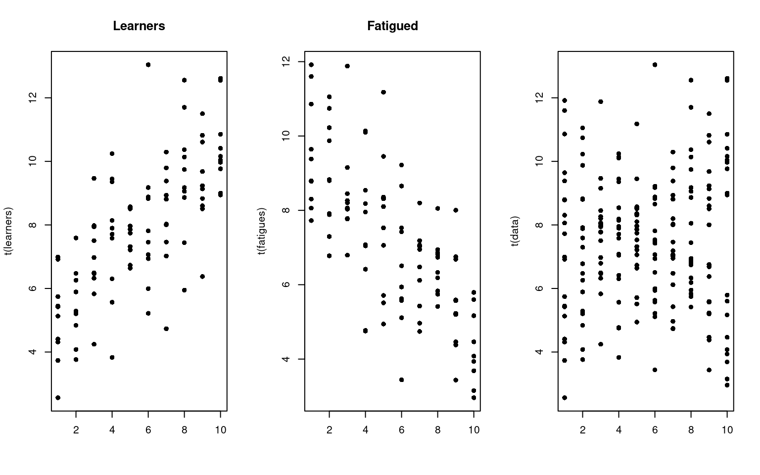

Although we have two different groups, without knowing about their identity, we might just look at the data and declare that they are all the same. Of course, if they were all the same, we would see some that have a positive slope, and some that have a negative slope. Seeing some with positive and some with negative slope doesn’t necessarily tell us we have two groups though. For example, here is a a data set created from a single group

data2 <- matrix(5 + rnorm(200) * 2, 20)

pars1 <- matrix(0, ncol = 2, nrow = 20)
pars2 <- matrix(0, ncol = 2, nrow = 20)
pred <- 1:10
for (i in 1:20) {
    pars1[i, ] <- lm(data[i, ] ~ pred)$coef
    pars2[i, ] <- lm(data2[i, ] ~ pred)$coef
}

par(mfrow = c(1, 2))
plot(pars1, xlab = "intercepts", ylab = "slopes", main = "Two groups")
plot(pars2, xlab = "intercepts", ylab = "slopes", main = "One group")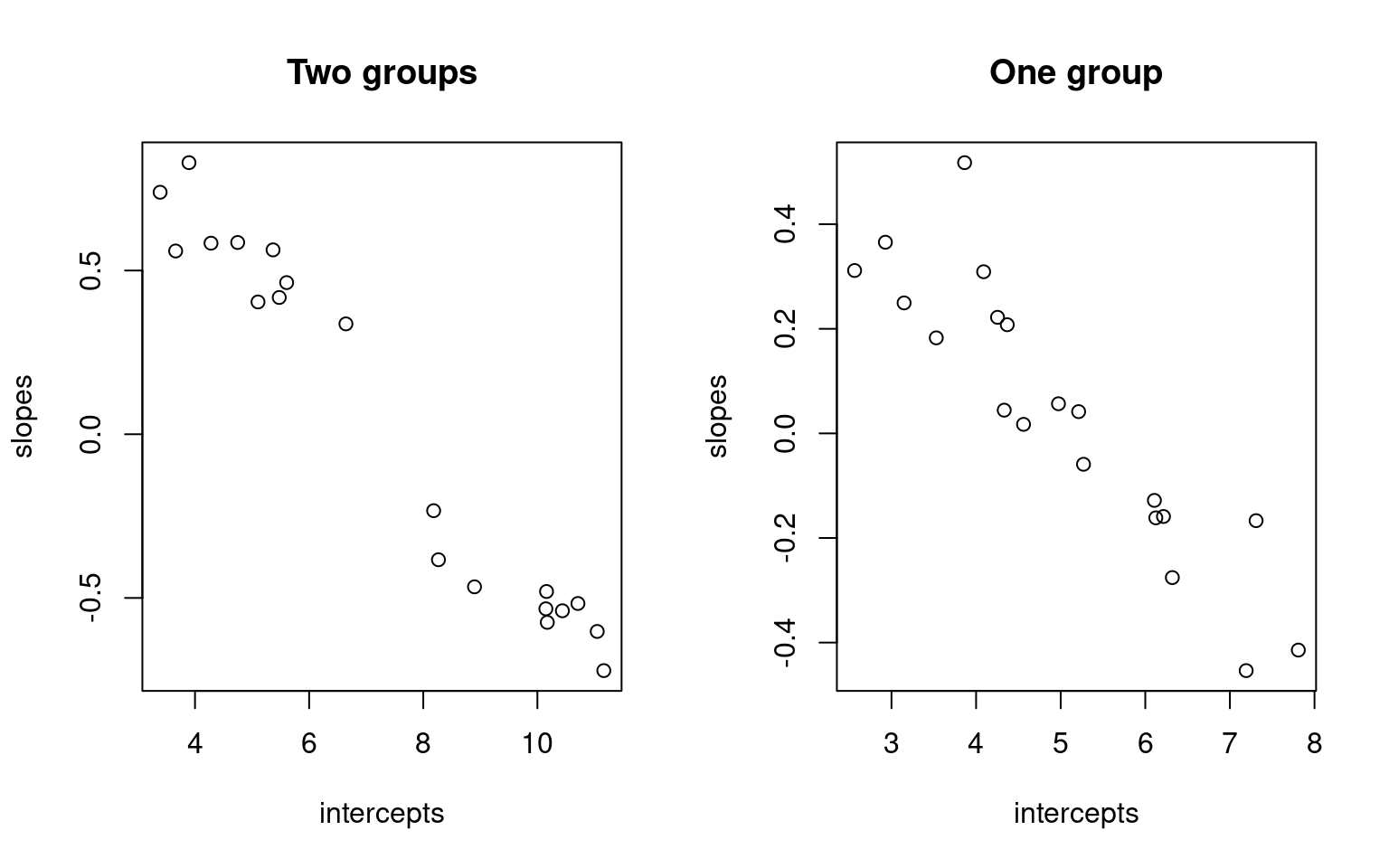

By comparing the slope and intercept of each person, we don’t see a lot of difference. But notice that when we have two groups, that if we fit a regression to each person, the resulting parameters appear to cluster into two groups, with a gap in the middle. When we have one group, they tend to vary more smoothly. A mixture model should be able to take advantage of this.

Howeever, to do so we need to reshape the data

library(reshape2)
data <- as.data.frame(data)
data$sub <- 1:20
long <- melt(data, id.vars = c("sub"))
long$time <- rep(1:10, each = 20)

long[1:10, ]

   sub variable    value time
1    1       V1 2.561813    1
2    2       V1 5.422148    1
3    3       V1 4.410111    1
4    4       V1 4.313140    1
5    5       V1 3.733472    1
6    6       V1 6.992038    1
7    7       V1 5.745078    1
8    8       V1 5.129919    1
9    9       V1 6.918519    1
10  10       V1 5.451357    1

Here, each predictor variable and subject are fitted separately. Now, we can make a repeated-measures regression with the following formula, which will aggregate across subject–exactly what we want. The points of each subject are classified all-or-none into one or the other cluster.

f <- flexmix(value ~ time | as.factor(sub), data = long, k = 2, control = list(iter.max = 10))
parameters(f)

                    Comp.1     Comp.2
coef.(Intercept) 4.8171232  9.9187058
coef.time        0.5481169 -0.5051437
sigma            1.5262642  1.4203917

clusters(f)

 [1] 1 1 1 1 1 1 1 1 1 1 2 2 2 2 2 2 2 2 2 2 1 1 1 1 1 1 1 1 1 1 2 2 2 2 2 2 2 2
[39] 2 2 1 1 1 1 1 1 1 1 1 1 2 2 2 2 2 2 2 2 2 2 1 1 1 1 1 1 1 1 1 1 2 2 2 2 2
 [ reached getOption("max.print") -- omitted 125 entries ]

table(clusters(f), long$sub)

   
     1  2  3  4  5  6  7  8  9 10 11 12 13 14 15 16 17 18 19 20
  1 10 10 10 10 10 10 10 10 10 10  0  0  0  0  0  0  0  0  0  0
  2  0  0  0  0  0  0  0  0  0  0 10 10 10 10 10 10 10 10 10 10

f1 <- flexmix(value ~ time | as.factor(sub), data = long, k = 1, control = list(iter.max = 10))

Example: Curved versus straight models

Mixtures don’t always come from the same process or type of model. Here is a one in which one component is linear, and a second is curved.

x1 <- rnorm(1000) * 5
x2 <- rnorm(1000) * 5
y1 <- 3 * x1 + 10 + rnorm(1000) * 5
y2 <- 10 + 5 * x2 + 0.3 * x2^2 + rnorm(1000) * 5
x <- c(x1, x2)
y <- c(y1, y2)
plot(x, y)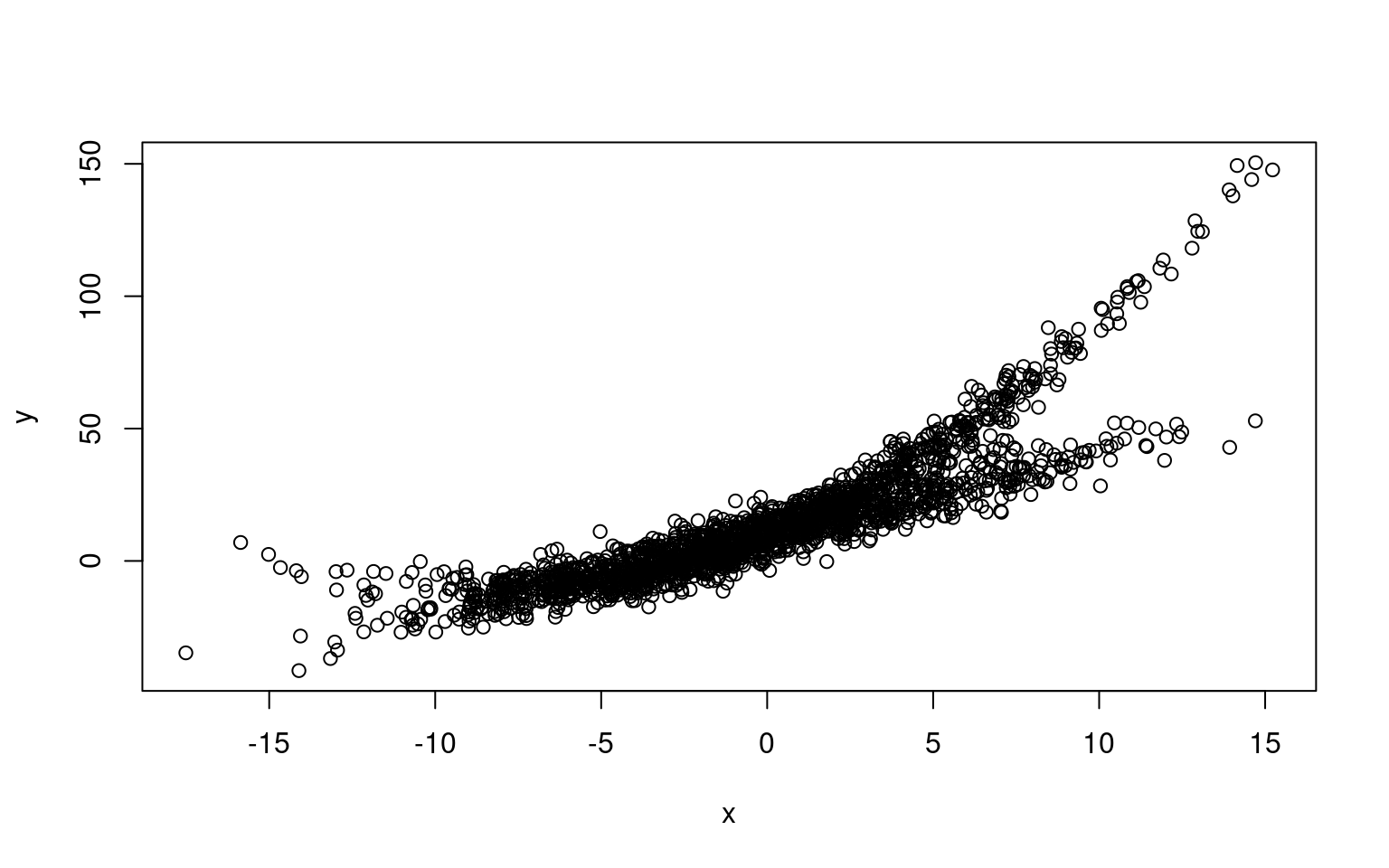

Here, we fit two polynomial models, this might work, because a linear model is just a subset of a polynomial model

model3 <- flexmix(y ~ poly(x, 2), k = 2)
summary(model3)


Call:
flexmix(formula = y ~ poly(x, 2), k = 2)

       prior size post>0 ratio
Comp.1 0.505  926   1872 0.495
Comp.2 0.495 1074   1877 0.572

'log Lik.' -6438.9 (df=9)
AIC: 12895.8   BIC: 12946.21

plot(x, y, col = c("red", "green")[clusters(model3)])

ord <- order(x)
points(x[ord], predict(model3)[[1]][ord], type = "l", col = "black", lwd = 6)
points(x[ord], predict(model3)[[1]][ord], type = "l", col = "red", lwd = 3)
points(x[ord], predict(model3)[[2]][ord], type = "l", col = "black", lwd = 6)
points(x[ord], predict(model3)[[2]][ord], type = "l", col = "green", lwd = 3)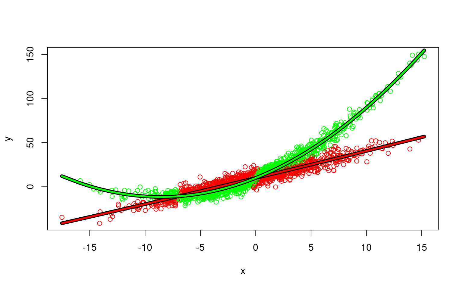

We can look at basic statistical tests with the following trick:

model3 <- flexmix(y ~ poly(x, 2), k = 2)
rm1 <- refit(model3)
summary(rm1)

$Comp.1
              Estimate Std. Error z value  Pr(>|z|)    
(Intercept)   16.73154    0.23836  70.195 < 2.2e-16 ***
poly(x, 2)1 1117.82809    8.45443 132.218 < 2.2e-16 ***
poly(x, 2)2  463.06664    7.56269  61.230 < 2.2e-16 ***
---
Signif. codes:  0 '***' 0.001 '**' 0.01 '*' 0.05 '.' 0.1 ' ' 1

$Comp.2
            Estimate Std. Error z value Pr(>|z|)    
(Intercept)   9.6721     0.2387  40.520   <2e-16 ***
poly(x, 2)1 677.3607     8.9369  75.794   <2e-16 ***
poly(x, 2)2   7.1761     8.6461   0.830   0.4066    
---
Signif. codes:  0 '***' 0.001 '**' 0.01 '*' 0.05 '.' 0.1 ' ' 1

You can see that for one model, it is quadratic, but for the other the quadratic term is not significant.

Control parameters

If you want to set a maximum number of iterations = 10 in model3,

>model31 <- flexmix(y~poly(x,2),k=2,control = list(iter.max=10))

Another control parameter is minprior. it is the minimum prior probability that components are enforced to have. Components falling below this threshold (the current default is 0.05) are removed during EM iteration to avoid numerical instabilities for components containing only a few observations. Using a minimum prior of 0 disables component removal. Here is a regression model with two latent classes. We can compare it to the actual class at the end:

data("NPreg")
m1 <- flexmix(yp ~ x + I(x^2), data = NPreg, k = 4, control = list(minprior = 0.2))
summary(m1)


Call:
flexmix(formula = yp ~ x + I(x^2), data = NPreg, k = 4, control = list(minprior = 0.2))

       prior size post>0 ratio
Comp.1  0.48   78    200 0.390
Comp.2  0.52  122    180 0.678

'log Lik.' -439.1561 (df=9)
AIC: 896.3123   BIC: 925.9971

plot(m1)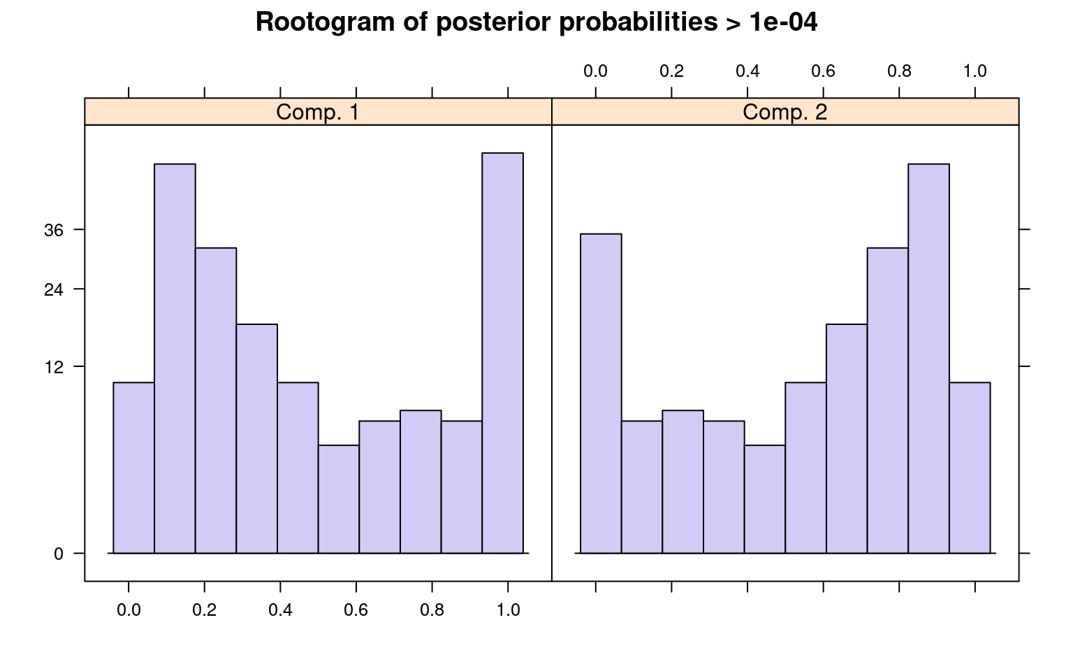

clusters(m1)

 [1] 2 2 1 2 2 2 2 2 2 2 2 2 1 2 2 1 2 2 2 1 1 1 2 1 2 2 2 2 2 1 2 1 1 1 2 2 2 1
[39] 1 2 2 1 2 2 2 2 2 2 2 1 2 2 2 2 2 1 2 1 2 2 2 1 2 1 2 2 2 2 2 2 2 2 1 2 2
 [ reached getOption("max.print") -- omitted 125 entries ]

table(NPreg$class, clusters(m1))

Model-based classification and semi-supervised classification.

Many of the model-based clustering libraries, including mclust, have capabilities for doing model-based classification and semi-supervised classification. You can think of classification and clustering on two ends of a spectrum–when you know the answer and when you do not know the answer. Mid-points include when you know the answers of only SOME of the cases, and when you know answers for all or some of the cases but only probabilistically. These frameworks integrate classification and clustering under one approach. For mclust, there are two related functions:

MClustSSC: This performs semi-supervised clustering. It STARTS with the labeled data as the initial clusters, but then performs the normal EM algorithm and reclassifies each element based on an evolving set of clusters.
MClustDA: Cluster-based LDA. This is much more like traditional LDA, but you can specify each of the different kinds of gaussian models (constraining variance, covarience, volume, etc.)

Cluster-based discriminant analysis.

For the discriminant analysis, suppose we have two groups that are not well defined by a single gaussian, but rather one is a ‘peanut’

library(ggplot2)
library(mclust)

groupA <- rbind(cbind(x = rnorm(100, mean = 30, sd = 5), y = rnorm(100, mean = 80,
    sd = 5)), cbind(x = rnorm(100, mean = 60, sd = 5), y = rnorm(100, mean = 80,
    sd = 5)))
groupB <- cbind(x = rnorm(200, mean = 30, sd = 10), y = rnorm(200, mean = 60, sd = 10))


dat <- data.frame(group = rep(c("A", "B"), each = 200), x = c(groupA[, 1], groupB[,
    1]), y = c(groupA[, 2], groupB[, 2]))

dat |>
    ggplot(aes(x = x, y = y, color = group)) + geom_point() + theme_bw()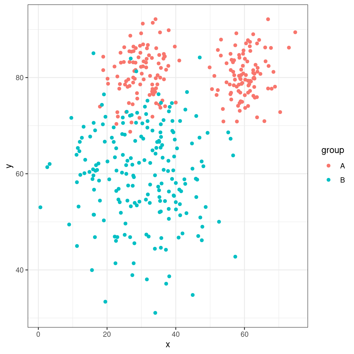

model <- MclustDA(dat[, 2:3], dat$group)

plot(model, "classification")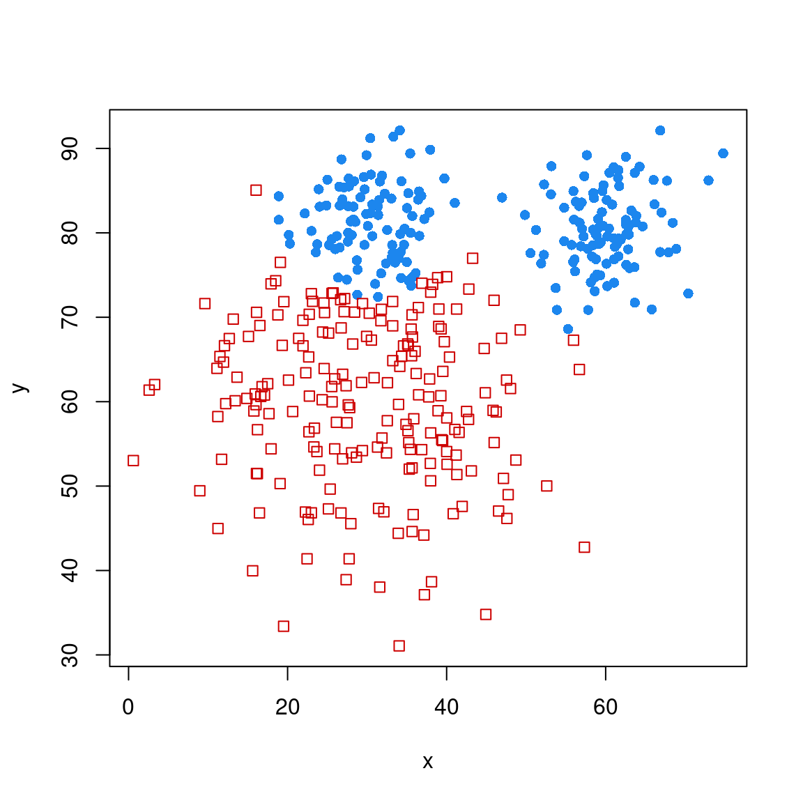

plot(model, "scatterplot")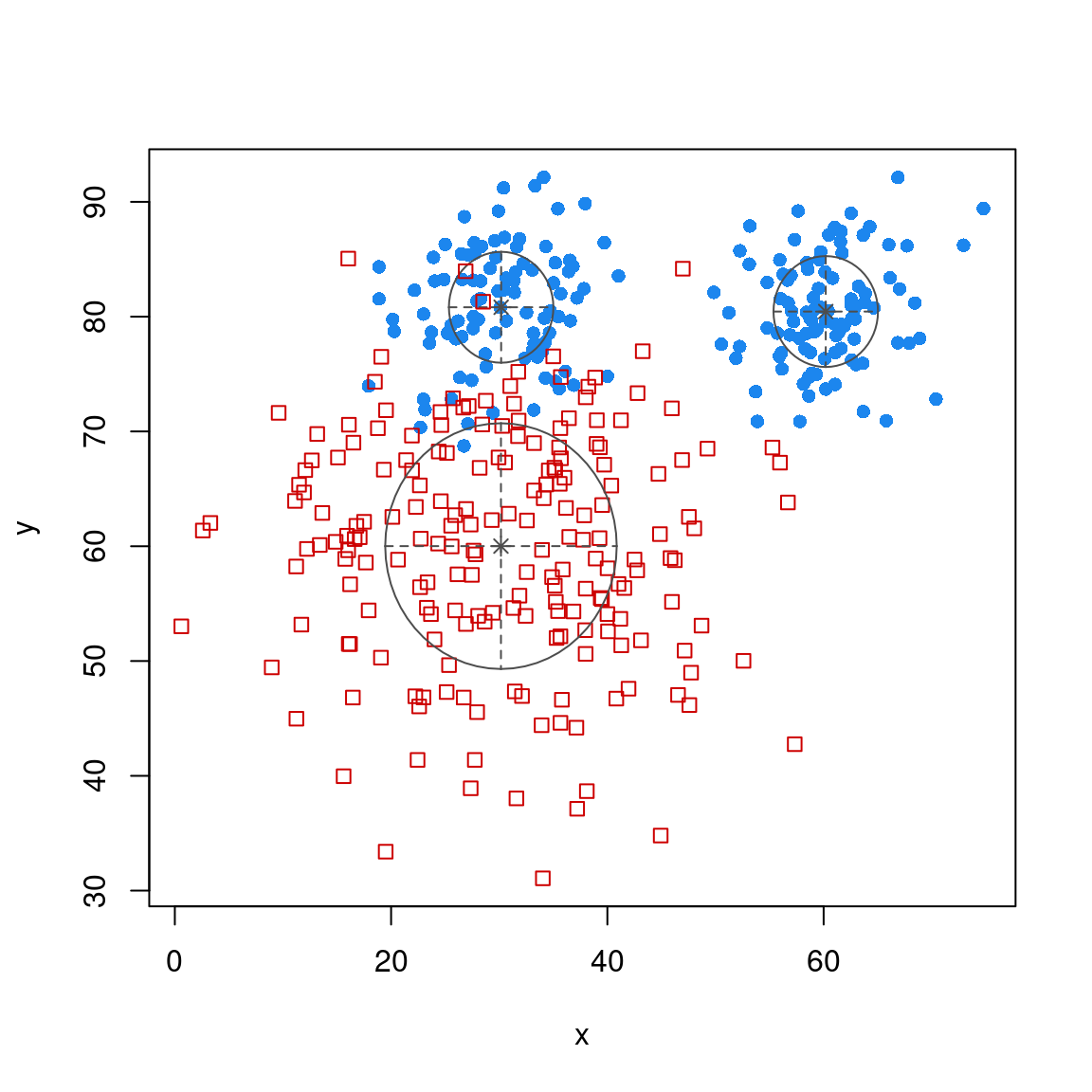

summary(model)

------------------------------------------------ 
Gaussian finite mixture model for classification 
------------------------------------------------ 

MclustDA model summary: 

 log-likelihood   n df       BIC
      -3078.028 400  9 -6209.979
       
Classes   n  % Model G
      A 200 50   EII 2
      B 200 50   XII 1

Training confusion matrix:
     Predicted
Class   A   B
    A 189  11
    B  10 190
Classification error = 0.0525 
Brier score          = 0.0379

Notice that the MclustDA allows multiple gaussians to describe groups. It does its own leave-one-out cross-validation, and determines an error rate of around 7%. You can use it to make a prediction about a new data set or observation as well:

predict(model, newdata = data.frame(x = 0.5, y = 0.5))

$classification
[1] B
Levels: A B

$z
                A B
[1,] 3.529834e-60 1

This LDA not only permits multiple clusters, but gaussians of any of the shapes we considered in the clustering technique. This gives the model a lot of power to describe arbitrarily complex classes.

Semi-supervised clustering

Semi-supervised clustering is often used for cases in which you have labels for a few cases, but most cases are unlabelled. In our data set above, let’s pick just a few:

dat$label <- NA
dat$label[1:3] <- "PEANUT"
dat$label[101:103] <- "PEANUT"
dat$label[201:203] <- "OREO"

partialmodel1 <- MclustSSC(dat[, 2:3], dat$label)
summary(partialmodel1)

---------------------------------------------------------------- 
Gaussian finite mixture model for semi-supervised classification 
---------------------------------------------------------------- 

 log-likelihood   n df       BIC
      -3159.963 400  9 -6373.848
        
Classes    n     % Model G
  OREO     3  0.75   VVI 1
  PEANUT   6  1.50   VVI 1
  <NA>   391 97.75        

Classification summary:
        Predicted
Class    OREO PEANUT
  OREO      3      0
  PEANUT    0      6
  <NA>    219    172

plot(partialmodel1, "uncertainty")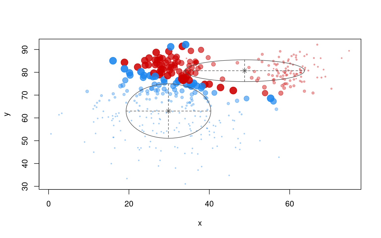

plot(partialmodel1, "classification")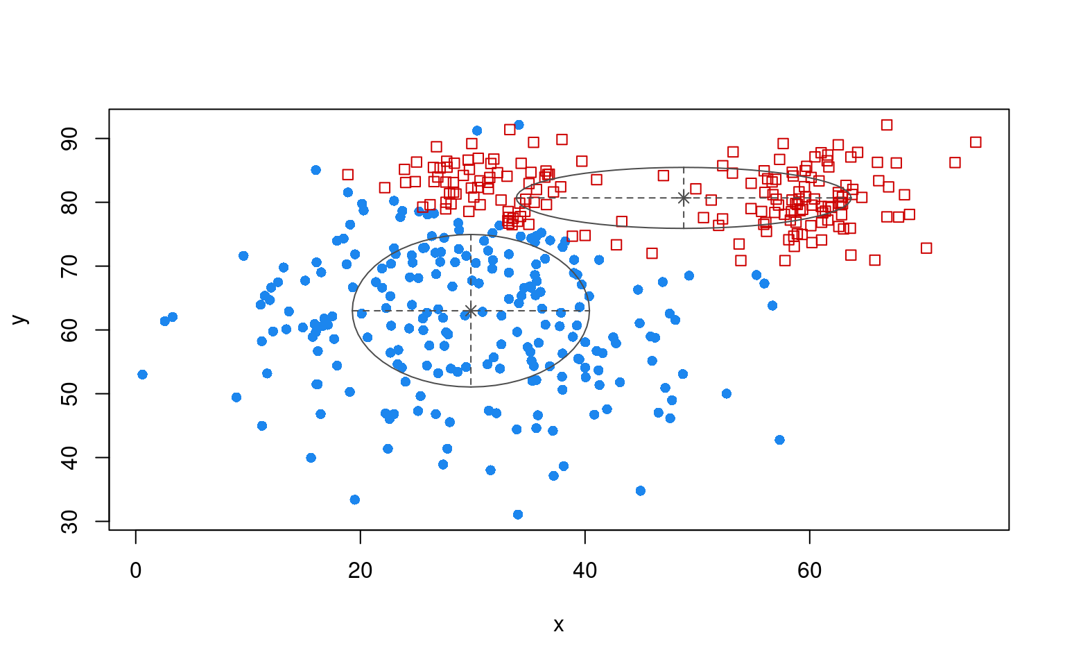

table(dat$group, partialmodel1$classification)

   
    OREO PEANUT
  A   30    170
  B  192      8

In this case, we don’t do very well, because the even though the two pods of the peanut had labelled cases, they get put into different clusters. The EM is performed without regard to accuracy; it only starts out correctly. Furthermore, unlike the LDA application, it will not assign a single label to multiple clusters. What if we forced it to use three clusters?

## FORCE IT TO USE THREE LATENT CLUSTERS:
partialmodel2 <- MclustSSC(dat[, 2:3], dat$label, G = 3)
summary(partialmodel2)

---------------------------------------------------------------- 
Gaussian finite mixture model for semi-supervised classification 
---------------------------------------------------------------- 

 log-likelihood   n df       BIC
      -3122.516 400  8 -6292.964
        
Classes    n     % Model G
  OREO     3  0.75   VII 1
  PEANUT   6  1.50   VII 1
  class3   0  0.00   VII 1
  <NA>   391 97.75        

Classification summary:
        Predicted
Class    OREO PEANUT class3
  OREO      3      0      0
  PEANUT    0      6      0
  <NA>    197    100     94

plot(partialmodel2, "uncertainty")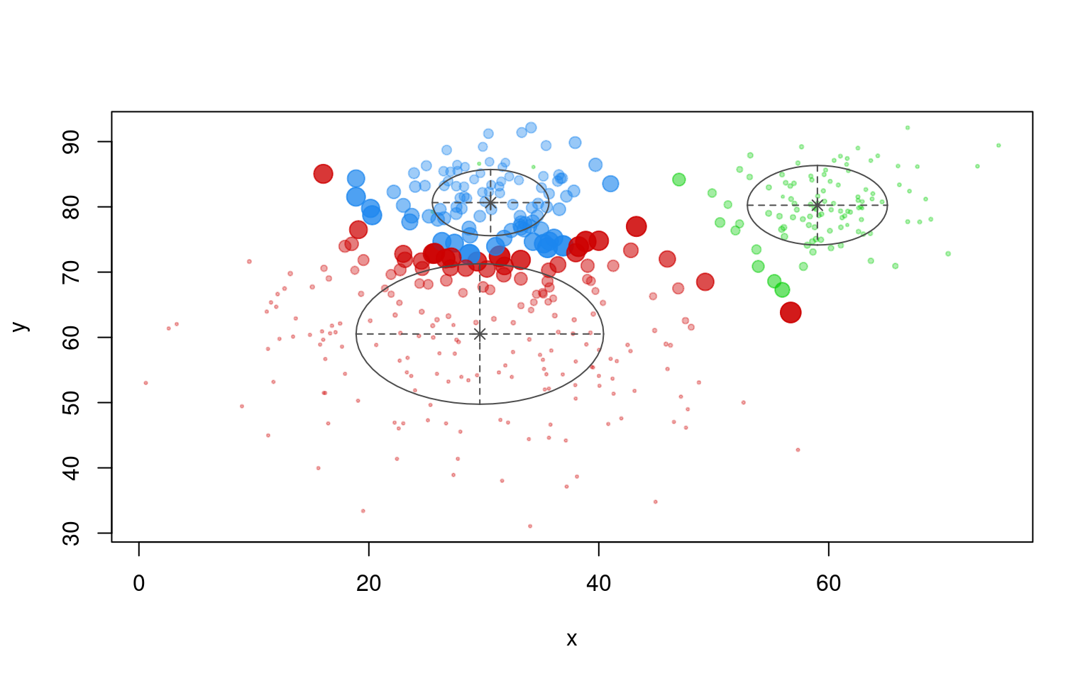

plot(partialmodel2, "classification")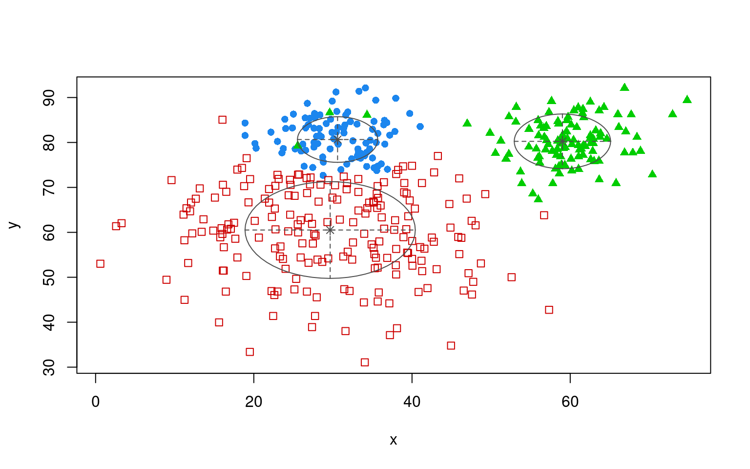

table(dat$group, partialmodel2$classification)

   
    OREO PEANUT class3
  A   10    103     87
  B  190      3      7

This is not bad, but it infers a ‘class3’ label that is actually the peanut group. Several of the other EM clustering techniques provide other partially-supervised algorithms, and those might in fact be more flexible that this particular one.

Summary

In this module, we learned about extending model-based clustering to regression and classification problems. We used flexmix to build arbitrary mixtures of regressions, and explored an interesting classification method with mclust using mixtures of guassians. Finally, we examined a situation where we have a small number of labelled cases and we want to use that to label the clusters that emerge.

References

Leisch, F. (2004). Flexmix: A general framework for finite mixture models and latent class regression in R. Journal of Statistical Software, 1-18.

Mixture Modeling: Mixture of Regressions