Exploratory Factor Analysis
Exploratory Factor analysis
Some resources:
Libraries used:
psychGPArotationfactoextra
PCA and SVD are considered simple forms of exploratory factor analysis. The term ‘factor analysis’ is a bit confusing and you will find a variety of definitions out there–some people assert that PCA is not factor analysis, and others might use PCA but call it factor analysis. Remember that PCA involves a complete redescription of the covariance or correlation matrix along a set of independent dimensions using Eigen decomposition, until they completely redescribe the data. Eigen decomposition ranks the dimensions by the variance, and so there is a fall-off in how useful consecutive dimensions are. We usually pick off the most important components and ignore the rest, treating them as noise. But if we think about what we learned with cluster analysis and MDS, sometimes there are unique but important low-level aspects of variance that might be better to incorporate into our components. MDS does this by forcing the distance space into a fixed number of dimensions. Similarly, factor analysis tries to fit a model of a fixed number of dimensions or factors. It does this by trying to maximize the variance accounted for by a fixed number of ‘latent’ factors, so that we have a deliberate model + error approach. In any case, like PCA factor analysis involves modeling the covariance or correlation matrix, and is an example of a broader set of approaches called ‘covariance models’.
Making an analogy to MDS, classic MDS used eigen decomposition and then peels off just the top dimensions. But sammon and non-metric scaling try to force the higher dimensions into fewer. Now, instead of fitting all the noise, we can minimize or optimize some notion of fitting the correlation matrix, and treat everything else as noise. When an algorithm has this goal, it is typically called ‘factor analysis’. As such, it is important when you report an analysis to give specific details of how the analysis was performed, including the software routine and arguments used.
A simple example
In the section on PCA, we examined human abilities and came up with a solution in which one component was an overall ability across all skills, one was visual vs. verbal, and a third was picture vs. maze:
library(GPArotation)
# library(psych)
data(ability.cov)
e2 <- eigen(cov2cor(ability.cov$cov))
plot(e2$values)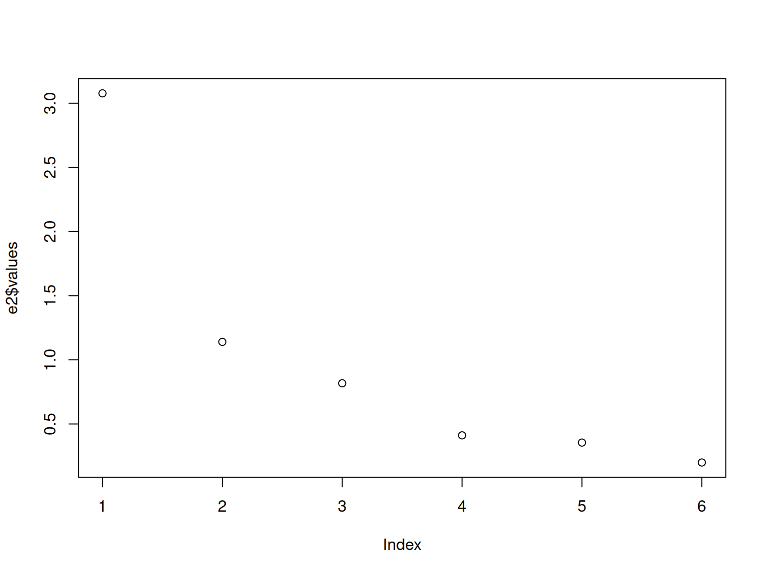
          [,1]   [,2]   [,3]   [,4]   [,5]   [,6]
general -0.471  0.002  0.072  0.863  0.037 -0.164
picture -0.358  0.408  0.593 -0.268  0.531  0.002
blocks  -0.434  0.404  0.064 -0.201 -0.775  0.051
maze    -0.288  0.404 -0.794 -0.097  0.334  0.052
reading -0.440 -0.507 -0.015 -0.100  0.056  0.733
vocab   -0.430 -0.501 -0.090 -0.352  0.021 -0.657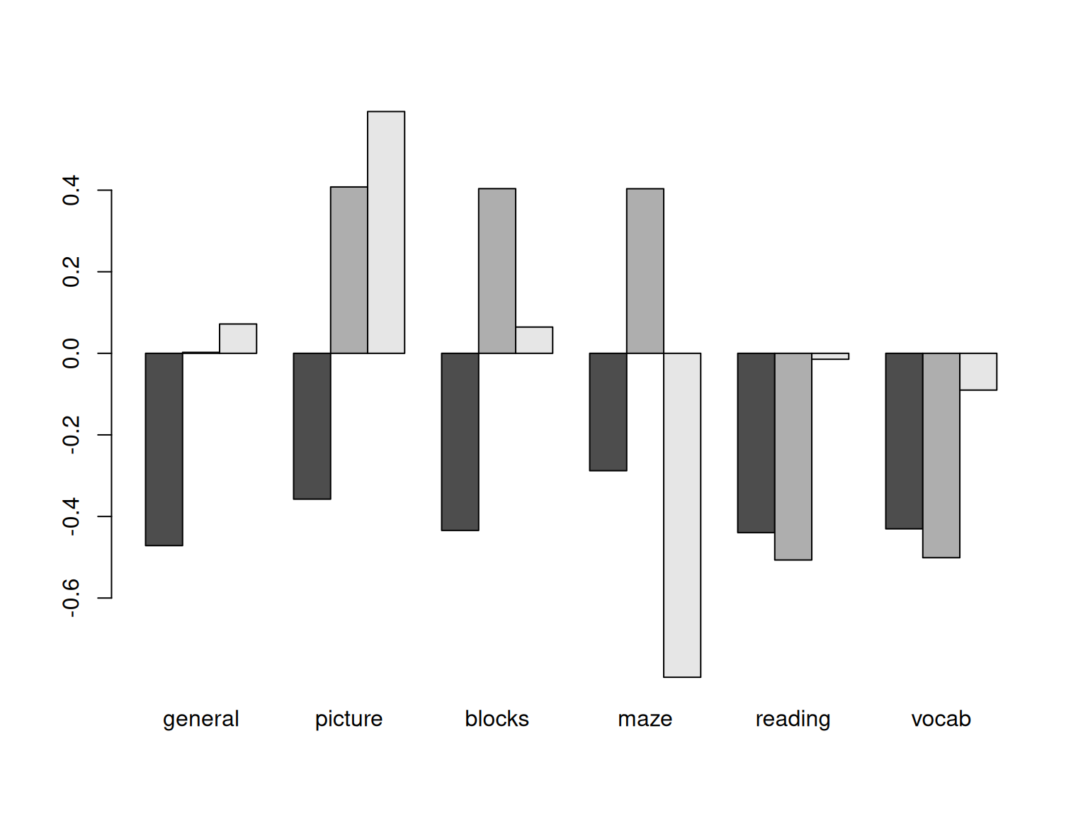
We can use the factanal function to do something
similar, giving it the covariance matrix. We now specify exactly how
many factors we want:
Call:
factanal(factors = 3, covmat = ability.cov)

Uniquenesses:
general picture  blocks    maze reading   vocab
  0.441   0.217   0.329   0.580   0.040   0.336

Loadings:
        Factor1 Factor2 Factor3
general 0.499   0.394   0.393
picture 0.133   0.862   0.153
blocks  0.230   0.525   0.586
maze    0.110           0.632
reading 0.965   0.138   0.102
vocab   0.782   0.123   0.192

               Factor1 Factor2 Factor3
SS loadings      1.874   1.217   0.967
Proportion Var   0.312   0.203   0.161
Cumulative Var   0.312   0.515   0.676

The degrees of freedom for the model is 0 and the fit was 0 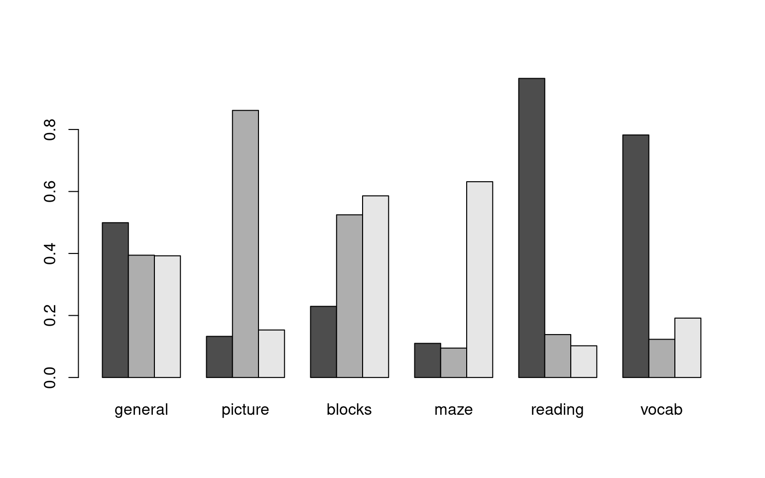 Now, the first three factors turn out a bit differently. factor1 is the
specific
Now, the first three factors turn out a bit differently. factor1 is the
specific general skill, reading and vocab–a basic verbal
ability. Factor 2 is picture+books; the visual skills that don’t involve
maze, plus some general. The third loads highly on blocks, maze, and
general. These tend to focus on single common positively-correlated
factors rather than the divisive components we happened to get with PCA.
If you think about it, a mixture of these three factors can produce
basically the same patterns as the first three factors of the PCA, but
in a different way. Note that the PCA dimensions do not change as we
increase the number of dimensions–we do this once and pick off the first
few dimensions we care about. FA gives us the best model with a limited
number of factors (usually from a maximum likelihood perspective), and
it calculates a statistical test asking whether the model is sufficient,
at least if it can compute this. For f3, it cannot be calculated, and it
says the DF of the model is 0 and the fit is 0. For 1- and 2-factor
models, it tells us that 1-factor fails but 2-factor does not,
suggesting a 2-factor solution is sufficient.
f1 <- factanal(covmat = ability.cov, factors = 1)
f2 <- factanal(covmat = ability.cov, factors = 2)

f1
Call:
factanal(factors = 1, covmat = ability.cov)

Uniquenesses:
general picture  blocks    maze reading   vocab
  0.535   0.853   0.748   0.910   0.232   0.280

Loadings:
        Factor1
general 0.682
picture 0.384
blocks  0.502
maze    0.300
reading 0.877
vocab   0.849

               Factor1
SS loadings      2.443
Proportion Var   0.407

Test of the hypothesis that 1 factor is sufficient.
The chi square statistic is 75.18 on 9 degrees of freedom.
The p-value is 1.46e-12
Call:
factanal(factors = 2, covmat = ability.cov)

Uniquenesses:
general picture  blocks    maze reading   vocab
  0.455   0.589   0.218   0.769   0.052   0.334

Loadings:
        Factor1 Factor2
general 0.499   0.543
picture 0.156   0.622
blocks  0.206   0.860
maze    0.109   0.468
reading 0.956   0.182
vocab   0.785   0.225

               Factor1 Factor2
SS loadings      1.858   1.724
Proportion Var   0.310   0.287
Cumulative Var   0.310   0.597

Test of the hypothesis that 2 factors are sufficient.
The chi square statistic is 6.11 on 4 degrees of freedom.
The p-value is 0.191
Each variable is given a ‘uniqueness’ score, which is the error variance of that term–the unique variance not accounted for by the model. This can help identify whether there are measures that should be removed, because they are simply multiple measures of the same thing. Also, the factors show sum-of-squares (variance), proportion and cumulative, to give a basic effect size for each factor. Because the factors try to maximize variance, we see less of a fall-off in explained variance across factors, and the method balances variance more equally across factors. However, as we increase the number of factors, you can see the total additional variance accounted for per dimension tends to gets smaller. In this case, f1 accounted for 41%, f2 accounted for 50%, and f3 accounted for 67%.
Now that we see some of the similarities and differences, let’s examine the different arguments to factor analysis.
Input data
factanal can use a formula with the raw data, or a covariance or correlation matrix. When given data, it will form the covariance matrix. When given a formula, you specify nothing to the left of the ~, but any variable you care about to the right. If no formula is given, it will use all the variables.
Notice that each of the following produces exactly the same results:
A <- rnorm(100)
B <- rnorm(100)
C <- A + rnorm(100) * 5
D <- B + rnorm(100) * 5
E <- A - B + rnorm(100) * 4
F <- C + D + rnorm(100) * 5
data <- data.frame(A, B, C, D, E, F)

factanal(data, factors = 3)
Call:
factanal(x = data, factors = 3)

Uniquenesses:
    A     B     C     D     E     F
0.937 0.791 0.453 0.005 0.005 0.005

Loadings:
  Factor1 Factor2 Factor3
A  0.201           0.135
B          0.438  -0.128
C  0.733
D  0.273   0.946   0.158
E  0.101  -0.121   0.985
F  0.939   0.322

               Factor1 Factor2 Factor3
SS loadings      1.545   1.219   1.039
Proportion Var   0.258   0.203   0.173
Cumulative Var   0.258   0.461   0.634

The degrees of freedom for the model is 0 and the fit was 0.0028
Call:
factanal(x = ~A + B + C + D + E + F, factors = 3, data = data)

Uniquenesses:
    A     B     C     D     E     F
0.937 0.791 0.453 0.005 0.005 0.005

Loadings:
  Factor1 Factor2 Factor3
A  0.201           0.135
B          0.438  -0.128
C  0.733
D  0.273   0.946   0.158
E  0.101  -0.121   0.985
F  0.939   0.322

               Factor1 Factor2 Factor3
SS loadings      1.545   1.219   1.039
Proportion Var   0.258   0.203   0.173
Cumulative Var   0.258   0.461   0.634

The degrees of freedom for the model is 0 and the fit was 0.0028
Call:
factanal(factors = 3, covmat = cov(data))

Uniquenesses:
    A     B     C     D     E     F
0.937 0.791 0.453 0.005 0.005 0.005

Loadings:
  Factor1 Factor2 Factor3
A  0.201           0.135
B          0.438  -0.128
C  0.733
D  0.273   0.946   0.158
E  0.101  -0.121   0.985
F  0.939   0.322

               Factor1 Factor2 Factor3
SS loadings      1.545   1.219   1.039
Proportion Var   0.258   0.203   0.173
Cumulative Var   0.258   0.461   0.634

The degrees of freedom for the model is 0 and the fit was 0.0028
Call:
factanal(factors = 3, covmat = cor(data))

Uniquenesses:
    A     B     C     D     E     F
0.937 0.791 0.453 0.005 0.005 0.005

Loadings:
  Factor1 Factor2 Factor3
A  0.201           0.135
B          0.438  -0.128
C  0.733
D  0.273   0.946   0.158
E  0.101  -0.121   0.985
F  0.939   0.322

               Factor1 Factor2 Factor3
SS loadings      1.545   1.219   1.039
Proportion Var   0.258   0.203   0.173
Cumulative Var   0.258   0.461   0.634

The degrees of freedom for the model is 0 and the fit was 0.0028
The psych library offers the fa() function
which has much more detailed output and other options. This function has
a lot of capabilities, but if we specify the varimax rotation, we get
nearly the same results:
Factor Analysis using method =  minres
Call: psych::fa(r = (data), nfactors = 3, rotate = "varimax")
Standardized loadings (pattern matrix) based upon correlation matrix
    MR1   MR3   MR2    h2     u2 com
A  0.20  0.08  0.13 0.064 0.9356 2.0
B -0.01  0.43 -0.13 0.202 0.7975 1.2
C  0.75 -0.10  0.00 0.572 0.4278 1.0
D  0.27  0.95  0.15 0.997 0.0033 1.2
E  0.11 -0.12  0.99 0.996 0.0038 1.1
F  0.92  0.33  0.09 0.960 0.0405 1.3

                       MR1  MR3  MR2
SS loadings           1.53 1.22 1.04
Proportion Var        0.26 0.20 0.17
Cumulative Var        0.26 0.46 0.63
Proportion Explained  0.40 0.32 0.27
Cumulative Proportion 0.40 0.73 1.00

Mean item complexity =  1.3
Test of the hypothesis that 3 factors are sufficient.

The degrees of freedom for the null model are  15  and the objective function was  1.51 with Chi Square of  144.89
The degrees of freedom for the model are 0  and the objective function was  0

The root mean square of the residuals (RMSR) is  0.01
The df corrected root mean square of the residuals is  NA

The harmonic number of observations is  100 with the empirical chi square  0.24  with prob <  NA
The total number of observations was  100  with Likelihood Chi Square =  0.36  with prob <  NA

Tucker Lewis Index of factoring reliability =  -Inf
Fit based upon off diagonal values = 1
Measures of factor score adequacy
                                                   MR1  MR3  MR2
Correlation of (regression) scores with factors   0.98 1.00 1.00
Multiple R square of scores with factors          0.95 1.00 0.99
Minimum correlation of possible factor scores     0.90 0.99 0.99
Because these different functions all end up calculating correlations, this means that missing data (with NA values) can be troublesome. To deal with it, you can specify an na.action, including imputing a prediction about the missing values or ignoring them. Alternately, you can handle this when you make the covariance or correlation matrix.
Factor Analysis using method =  minres
Call: fa(r = data, nfactors = 3)
Standardized loadings (pattern matrix) based upon correlation matrix
    MR1   MR3   MR2    h2     u2 com
A  0.18  0.07  0.11 0.064 0.9356 2.0
B -0.09  0.44 -0.19 0.202 0.7975 1.4
C  0.81 -0.22 -0.01 0.572 0.4278 1.1
D  0.04  0.98  0.02 0.997 0.0033 1.0
E  0.00  0.00  1.00 0.996 0.0038 1.0
F  0.88  0.21  0.02 0.960 0.0405 1.1

                       MR1  MR3  MR2
SS loadings           1.48 1.26 1.05
Proportion Var        0.25 0.21 0.17
Cumulative Var        0.25 0.46 0.63
Proportion Explained  0.39 0.33 0.28
Cumulative Proportion 0.39 0.72 1.00

 With factor correlations of
     MR1  MR3  MR2
MR1 1.00 0.37 0.14
MR3 0.37 1.00 0.05
MR2 0.14 0.05 1.00

Mean item complexity =  1.3
Test of the hypothesis that 3 factors are sufficient.

df null model =  15  with the objective function =  1.51 with Chi Square =  144.89
df of  the model are 0  and the objective function was  0

The root mean square of the residuals (RMSR) is  0.01
The df corrected root mean square of the residuals is  NA

The harmonic n.obs is  100 with the empirical chi square  0.24  with prob <  NA
The total n.obs was  100  with Likelihood Chi Square =  0.36  with prob <  NA

Tucker Lewis Index of factoring reliability =  -Inf
Fit based upon off diagonal values = 1
Measures of factor score adequacy
                                                   MR1  MR3  MR2
Correlation of (regression) scores with factors   0.98 1.00 1.00
Multiple R square of scores with factors          0.96 1.00 1.00
Minimum correlation of possible factor scores     0.91 0.99 0.99
## try missing data:
data$A[30] <- NA
# factanal(data,factors=3) ## this does not work
# factanal(data,factors=3,na.action=na.omit) ## also does not work
factanal(~A + B + C + D + E + F, data = data, factors = 3, na.action = na.omit) ##this does
Call:
factanal(x = ~A + B + C + D + E + F, factors = 3, data = data,     na.action = na.omit)

Uniquenesses:
    A     B     C     D     E     F
0.936 0.801 0.453 0.005 0.005 0.005

Loadings:
  Factor1 Factor2 Factor3
A  0.198           0.146
B          0.431  -0.111
C  0.733
D  0.269   0.946   0.166
E         -0.110   0.987
F  0.938   0.322   0.107

               Factor1 Factor2 Factor3
SS loadings      1.537   1.210   1.047
Proportion Var   0.256   0.202   0.174
Cumulative Var   0.256   0.458   0.632

The degrees of freedom for the model is 0 and the fit was 0.0022 Factor Analysis using method = minres
Call: fa(r = data, nfactors = 3)
Standardized loadings (pattern matrix) based upon correlation matrix
MR1 MR3 MR2 h2 u2 com
A 0.18 0.06 0.12 0.066 0.9341 2.1
B -0.09 0.44 -0.19 0.202 0.7976 1.4
C 0.81 -0.22 -0.01 0.567 0.4328 1.1
D 0.04 0.98 0.02 0.997 0.0032 1.0
E 0.00 0.00 1.00 0.996 0.0038 1.0
F 0.88 0.21 0.02 0.965 0.0347 1.1
MR1 MR3 MR2
SS loadings 1.49 1.26 1.05
Proportion Var 0.25 0.21 0.18
Cumulative Var 0.25 0.46 0.63
Proportion Explained 0.39 0.33 0.28
Cumulative Proportion 0.39 0.72 1.00
With factor correlations of
MR1 MR3 MR2
MR1 1.00 0.37 0.14
MR3 0.37 1.00 0.05
MR2 0.14 0.05 1.00
Mean item complexity = 1.3
Test of the hypothesis that 3 factors are sufficient.
df null model = 15 with the objective function = 1.51 with Chi Square = 145.07
df of the model are 0 and the objective function was 0
The root mean square of the residuals (RMSR) is 0.01
The df corrected root mean square of the residuals is NA
The harmonic n.obs is 100 with the empirical chi square 0.2 with prob < NA
The total n.obs was 100 with Likelihood Chi Square = 0.32 with prob < NA
Tucker Lewis Index of factoring reliability = -Inf
Fit based upon off diagonal values = 1
Measures of factor score adequacy
MR1 MR3 MR2
Correlation of (regression) scores with factors 0.98 1.00 1.00
Multiple R square of scores with factors 0.96 1.00 1.00
Minimum correlation of possible factor scores 0.92 0.99 0.99Optimization method.
Factor analysis can be thought of as a model of the correlation matrix using a fixed number of hidden or latent predictors to describe the data. How this works is that the factor analysis method essentially tries to do PCA using an iterative approximation, with the restriction that you are forced to use a fixed number of factors. After starting at some solution, it iteratively refines this to best describe the data better and maximize goodness of fit of the model or minimize error in order to best describe the covariance data. However, it is not always exactly clear what ‘best describe the data’ means. Some traditional methods are ‘minres’, maximum likelihood, and principal axes, but other methods are available for special cases, depending on the software. In general, choice of optimization method probably depends more on requirements such as size, missing values, availability in the software you are using, etc. The results might not differ much, one probably won’t be universally better for all data sets, and results will be more impacted by other things such as the rotation. The literature suggests that the particular optimization methods differ across software packages, are not well documented, and typically produce similar results. Most sources appear to recommend using ML as a default if the matrix is well-behaved, and if it is not (i.e., the model does not converge) to try another method. The ML (maximum likelihood) factor analysis attempts to find a solution that is most likely to have produced the correlation matrix. Some methods will warn about ‘Heywood cases’ which could signal that another optimization method could be tried.
The factanal function in R uses ML and has a number of
options for controlling the estimation; the fa function in in the psych
offers more alternatives to ML, but its ML implementation has fewer
options. We will also use the psych::fa function because of better
output, but you might try an alternate implementation if you run into
trouble.
Rotations
Once a solution has been produced, we will have a small fixed number of components/factors that hopefully do a good job a redescribing the complete correlation matrix. But we have a potential problem of non-identifiability. These base factors will be orthogonal just as in PCA, which means that any point (i.e, a response pattern across questions) can be described as a combination of factors. But there are rotations of these axes that produce equally good fits. Thus, once the analysis is done, one usually chooses one of a number of rotations for looking at the data. Some common ones are available within the GPArotation library in R, and can be applied either as a function of fa, or afterward.
It might seem non-intuitive that the rotation is not a part of the optimizization. But unlike PCA which has a very well-defined way of assigning dimensions (each dimension maximizes variance in that direction, subject to being orthogonal to all others), factor analysis finds its solution to minimize residual variance/maximize goodness-of-fit. Consequently, it is more like MDS, in that a particular dimension that it picks may not be the best or most meaningful dimension to look at. A specific rotation may help, and often leads to more interpretable factors, because they are designed to hang together better and account for distinct variance. These rotations are available within several packages, including GPArotation, which is used by psych::fa.
varimax (variance maximizing rotation). This maximizes the variance of the factors. Because variance involves squared deviation, it is best to try to put all the variance of any question into a single factor, rather than spreading it out. So overall, factors should favor all-or-none membership of items. Thus it tries to align factors with measures that vary. This is the most popular orthogonal rotation method used frequently by default, and aims to find a simple model where questions are related to unique factors. Within psych::fa, it is no longer the default; as that package uses a non-orthogonal rotation.
quartimax. This maximizes the variance in each item (rather than each factor). Again, this aims for a simple model. To maximize the variance of each item, it should also be placed in a single factor, so it is described as minimizing the number of factors an item appears in.
equamax uses a weighted sum of varimax and quartimax.
varimin a does the opposite of what varimax does. It tries to minimize the variance of each item, so that each item is spread out across factors. This is useful when you have a lot of items that are not well described by a single factor.
geominT is a compromise between varimax and quartimax, and is often used when you have a lot of items that are not well described by a single factor.
bifactor is a special rotation that is used when you have a general factor and a number of specific factors. It is used to separate the general and specific factors. This is a special case of the oblique rotations, and is used when you have a general factor that is correlated with all the other factors.
A list of available orthogonal rotations includes: “none”, “varimax”, “quartimax”, “bentlerT”, “equamax”, “varimin”, “geominT” and “bifactor”
The above are all ‘orthogonal’ rotations–they require the factors to be independent and at right angles to one another. But it may be better if we allow the factors to be somewhat correlated if they are able to simplify the model more. These are not exactly rotations, because they are also essentially warping the dimensions of the space. They are more properly called ‘oblique transformations’.
The oblique transformations are harder to easily describe. They use differing criteria to try to create simple and interpretable models. For oblique transformations, the factors will be correlated with one another. However, the correlation cannot be too large, because then it would be better to combine those factors into a single factor.
Some options include the following. These are not well documented, and so it is usually preferable to use one that is well understood than to use one you cannot justify, but sometimes an exotic rotation will show a view of your data you did not see anywhere else. Many of the orthogonal rotations have oblique versions, where the orthogonal rotation ends with a T and the oblique ends with a Q.
- oblimin (default of the fa function).
- promax: an oblique transformation that has been described as having similar goals to varimax.
- simplimax: a simple structure oblique transformation that tries to maximize the variance of each item on a single factor.
- bentlerQ: a transformation that tries to maximize the variance of each item on a single factor, but also tries to minimize the number of factors each item appears in.
- geominQ: an oblique geomin.
- quartimin: a transformation that tries to minimize the variance of each item on a single factor.
- cluster: a transformation that tries to group items into clusters that are highly correlated with one another, but not with other clusters.
Example: Big Five data set
Let’s try reading in the big-five data set and performing a factor analysis with various different rotations. We will use the big five data, and both fa and factanal will take the entire data set directly, and not require you to compute a correlation matrix first.
Read in the big-five data set:
data <- read.csv("bigfive.csv")

dat.vals <- data[, -1]  ##remove subject code
qtype <- c("E", "A", "C", "N", "O", "E", "A", "C", "N", "O", "E", "A", "C", "N",
    "O", "E", "A", "C", "N", "O", "E", "A", "C", "N", "O", "E", "A", "C", "N", "O",
    "E", "A", "C", "N", "O", "E", "A", "C", "N", "O", "O", "A", "C", "O")
valence <- c(1, -1, 1, 1, 1, -1, 1, -1, -1, 1, 1, -1, 1, 1, 1, 1, 1, -1, 1, 1, -1,
    1, -1, -1, 1, 1, -1, 1, 1, 1, -1, 1, 1, -1, -1, 1, -1, 1, 1, 1, -1, 1, -1, 1)
add <- c(6, 0, 0)[valence + 2]


tmp <- dat.vals
tmp[is.na(tmp)] <- 3.5
reversed <- t(t(tmp) * valence + add)
## reverse code questions:

bytype <- reversed[, order(qtype)]
key <- sort(qtype)
colnames(bytype) <- paste(key, 1:44, sep = "")
#Factor analysis functions
First, let’s confirm that the different fa methods can produce similar results:
Call:
factanal(x = bytype, factors = 3)

Uniquenesses:
   A1    A2    A3    A4    A5    A6    A7    A8    A9   C10   C11   C12   C13
0.859 0.772 0.844 0.883 0.912 0.896 0.748 0.840 0.829 0.766 0.833 0.768 0.836
  C14   C15   C16   C17   C18   E19   E20   E21   E22   E23   E24   E25   E26
0.820 0.770 0.797 0.815 0.835 0.450 0.521 0.589 0.502 0.447 0.734 0.599 0.543
  N27   N28   N29   N30   N31   N32   N33   N34   O35   O36   O37   O38   O39
0.633 0.661 0.663 0.614 0.656 0.727 0.799 0.707 0.674 0.691 0.753 0.667 0.728
  O40   O41   O42   O43   O44
0.738 0.984 0.685 0.912 0.797

Loadings:
    Factor1 Factor2 Factor3
A1   0.367
A2   0.276   0.386
A3   0.328   0.125  -0.181
A4   0.250   0.233
A5   0.199   0.200
A6   0.278   0.105   0.125
A7   0.231   0.439
A8   0.354   0.160
A9   0.206   0.333   0.132
C10  0.277   0.397
C11  0.405
C12  0.278   0.393
C13  0.401
C14  0.398           0.121
C15  0.242   0.409
C16  0.299   0.318   0.111
C17  0.250   0.343
C18  0.403
E19          0.156   0.721
E20                  0.682
E21  0.205   0.287   0.535
E22  0.132   0.335   0.607
E23         -0.111   0.735
E24                  0.512
E25  0.236           0.585
 [ reached getOption("max.print") -- omitted 19 rows ]

               Factor1 Factor2 Factor3
SS loadings      4.219   3.854   3.631
Proportion Var   0.096   0.088   0.083
Cumulative Var   0.096   0.183   0.266

Test of the hypothesis that 3 factors are sufficient.
The chi square statistic is 5675.51 on 817 degrees of freedom.
The p-value is 0 Factor Analysis using method = minres
Call: fa(r = bytype, nfactors = 3, rotate = "varimax")
Standardized loadings (pattern matrix) based upon correlation matrix
MR1 MR2 MR3 h2 u2 com
A1 0.39 0.03 0.04 0.156 0.84 1.0
A2 0.33 0.38 0.02 0.250 0.75 2.0
A3 0.37 0.12 -0.22 0.197 0.80 1.9
A4 0.27 0.22 0.01 0.123 0.88 1.9
A5 0.23 0.18 0.07 0.091 0.91 2.2
A6 0.33 0.11 0.07 0.123 0.88 1.3
A7 0.29 0.44 -0.12 0.293 0.71 1.9
A8 0.40 0.16 -0.14 0.201 0.80 1.6
A9 0.25 0.33 0.10 0.178 0.82 2.1
C10 0.32 0.37 0.01 0.244 0.76 2.0
C11 0.44 0.00 -0.06 0.198 0.80 1.0
C12 0.34 0.37 -0.05 0.255 0.75 2.0
[ reached 'max' / getOption("max.print") -- omitted 32 rows ]
MR1 MR2 MR3
SS loadings 4.33 3.75 3.66
Proportion Var 0.10 0.09 0.08
Cumulative Var 0.10 0.18 0.27
Proportion Explained 0.37 0.32 0.31
Cumulative Proportion 0.37 0.69 1.00
Mean item complexity = 1.5
Test of the hypothesis that 3 factors are sufficient.
df null model = 946 with the objective function = 14.28 with Chi Square = 14284.11
df of the model are 817 and the objective function was 5.72
The root mean square of the residuals (RMSR) is 0.07
The df corrected root mean square of the residuals is 0.08
The harmonic n.obs is 1017 with the empirical chi square 9890.49 with prob < 0
The total n.obs was 1017 with Likelihood Chi Square = 5714.55 with prob < 0
Tucker Lewis Index of factoring reliability = 0.574
RMSEA index = 0.077 and the 90 % confidence intervals are 0.075 0.079
BIC = 57.14
Fit based upon off diagonal values = 0.83
Measures of factor score adequacy
MR1 MR2 MR3
Correlation of (regression) scores with factors 0.92 0.91 0.92
Multiple R square of scores with factors 0.84 0.83 0.85
Minimum correlation of possible factor scores 0.68 0.66 0.70
Notice that the two methods produce very similar results, but they display different information and show the factors differently. Let’s focus on the output of fa, which was done using the minres method; we could have also selected ml, wls, gls, or pa.
- It first shows a matrix that includes the three factors (MR2, MR3, and MR1), along with several other statistics. You can get this by doing loadings(model). This will display only the ‘important’ values–the values close to 0 will not be shown for easier examination.
- h2 is the communality score–sum of the squared factor loadings for each question. Somewhat like an \(R^2\) value for each item.
- u2 is the uniqueness score, 1-h2.
- com is complexity, an information score that is generally related to uniqueness.
Next, a number of statistics related to the model are shown. It then provides a chi-squared test of whether the model is sufficiently complex (or needs more factors), and other diagnostics of whether the model is acceptable. Because we guess there might be five, we will try five, using the ml optimization method
Optimization method
let’s look at different optimization methods, using the fm argument
Factor Analysis using method =  ml
Call: psych::fa(r = bytype, nfactors = 5, rotate = "quartimax", fm = "ml")
Standardized loadings (pattern matrix) based upon correlation matrix
     ML2   ML3   ML4   ML1   ML5   h2   u2 com
A1  0.10 -0.27 -0.05  0.08  0.33 0.20 0.80 2.3
A2  0.11 -0.07  0.17  0.34  0.35 0.29 0.71 2.7
A3 -0.13 -0.16 -0.04  0.15  0.43 0.25 0.75 1.8
A4  0.06 -0.13  0.11  0.17  0.29 0.14 0.86 2.5
A5  0.12 -0.06  0.05  0.26  0.17 0.11 0.89 2.5
A6  0.20 -0.09 -0.09  0.12  0.49 0.31 0.69 1.6
A7  0.00  0.02  0.18  0.28  0.57 0.43 0.57 1.7
A8 -0.04 -0.19  0.01  0.05  0.62 0.42 0.58 1.2
A9  0.19 -0.01  0.12  0.26  0.37 0.26 0.74 2.6
 [ reached 'max' / getOption("max.print") -- omitted 35 rows ]

                       ML2  ML3  ML4  ML1  ML5
SS loadings           3.60 3.42 3.19 2.89 2.40
Proportion Var        0.08 0.08 0.07 0.07 0.05
Cumulative Var        0.08 0.16 0.23 0.30 0.35
Proportion Explained  0.23 0.22 0.21 0.19 0.16
Cumulative Proportion 0.23 0.45 0.66 0.84 1.00

Mean item complexity =  1.8
Test of the hypothesis that 5 factors are sufficient.

df null model =  946  with the objective function =  14.28 with Chi Square =  14284.11
df of  the model are 736  and the objective function was  3.19

The root mean square of the residuals (RMSR) is  0.05
The df corrected root mean square of the residuals is  0.05

The harmonic n.obs is  1017 with the empirical chi square  4045.22  with prob <  0
The total n.obs was  1017  with Likelihood Chi Square =  3176.97  with prob <  3e-299

Tucker Lewis Index of factoring reliability =  0.764
RMSEA index =  0.057  and the 90 % confidence intervals are  0.055 0.059
BIC =  -1919.54
Fit based upon off diagonal values = 0.93
Measures of factor score adequacy
                                                   ML2  ML3  ML4  ML1  ML5
Correlation of (regression) scores with factors   0.93 0.92 0.91 0.88 0.88
Multiple R square of scores with factors          0.86 0.84 0.82 0.78 0.77
Minimum correlation of possible factor scores 0.73 0.68 0.65 0.56 0.53Factor Analysis using method = gls
Call: psych::fa(r = bytype, nfactors = 5, rotate = "quartimax", fm = "gls")
Standardized loadings (pattern matrix) based upon correlation matrix
GLS3 GLS4 GLS2 GLS5 GLS1 h2 u2 com
A1 0.11 -0.27 -0.08 0.06 0.41 0.26 0.74 2.0
A2 0.11 -0.06 0.19 0.31 0.40 0.31 0.69 2.6
A3 -0.15 -0.16 -0.03 0.14 0.48 0.29 0.71 1.6
A4 0.07 -0.12 0.11 0.12 0.37 0.18 0.82 1.8
A5 0.15 -0.04 0.04 0.23 0.25 0.14 0.86 2.8
A6 0.20 -0.08 -0.09 0.11 0.54 0.35 0.65 1.5
A7 0.00 0.02 0.23 0.23 0.56 0.42 0.58 1.7
A8 -0.06 -0.20 0.02 0.05 0.59 0.40 0.60 1.3
A9 0.21 0.00 0.15 0.22 0.41 0.28 0.72 2.5
[ reached 'max' / getOption("max.print") -- omitted 35 rows ]
GLS3 GLS4 GLS2 GLS5 GLS1
SS loadings 3.66 3.44 3.31 2.98 2.57
Proportion Var 0.08 0.08 0.08 0.07 0.06
Cumulative Var 0.08 0.16 0.24 0.30 0.36
Proportion Explained 0.23 0.22 0.21 0.19 0.16
Cumulative Proportion 0.23 0.44 0.65 0.84 1.00
Mean item complexity = 1.7
Test of the hypothesis that 5 factors are sufficient.
df null model = 946 with the objective function = 14.28 with Chi Square = 14284.11
df of the model are 736 and the objective function was 3.24
The root mean square of the residuals (RMSR) is 0.05
The df corrected root mean square of the residuals is 0.05
The harmonic n.obs is 1017 with the empirical chi square 4075.95 with prob < 0
The total n.obs was 1017 with Likelihood Chi Square = 3227.68 with prob < 9.7e-308
Tucker Lewis Index of factoring reliability = 0.759
RMSEA index = 0.058 and the 90 % confidence intervals are 0.056 0.06
BIC = -1868.83
Fit based upon off diagonal values = 0.93
Measures of factor score adequacy
GLS3 GLS4 GLS2 GLS5 GLS1
Correlation of (regression) scores with factors 0.93 0.92 0.92 0.90 0.90
Multiple R square of scores with factors 0.87 0.85 0.85 0.82 0.81
Minimum correlation of possible factor scores 0.73 0.70 0.70 0.63 0.62If you look at the loadings, values, etc. the factor analysis solutions are numerically different but tend to be fairly similar.
We can look at them specifically, especially in comparison to the PCA solution:
par(mfrow = c(3, 1))
matplot(loadings(f2), type = "s", lty = 1, main = "Factor analyis ML optimization")
matplot(loadings(f2b), type = "s", lty = 1, main = "Factor analysis GLS optimization")
matplot(loadings(pca)[, 1:5], main = "5 dimensions of PCA", type = "s", lty = 1)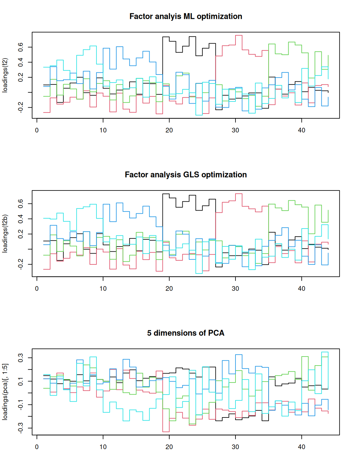 That does not look bad. If you compare to the factor loadings from the
PCA, these are much cleaner–the PCA is almost uninterpretable in
comparison. Notice that the two optimization methods produce results
that are essentially the same. It looks like each factor takes a turn
and maps roughly onto a different set of personality questions. This
structure comes from the quartimax rotation, not the optimization
method. But maybe other rotations would provide a stronger factor
structure. Although we applied rotations within the fa, we can also do
it afterward:
That does not look bad. If you compare to the factor loadings from the
PCA, these are much cleaner–the PCA is almost uninterpretable in
comparison. Notice that the two optimization methods produce results
that are essentially the same. It looks like each factor takes a turn
and maps roughly onto a different set of personality questions. This
structure comes from the quartimax rotation, not the optimization
method. But maybe other rotations would provide a stronger factor
structure. Although we applied rotations within the fa, we can also do
it afterward:
library(GPArotation)  ##needed for rotations like oblimin
matplot(varimax(loadings(f2))$loadings, type = "s", lty = 1, main = "varimax rotation",
    ylab = "Factor loading")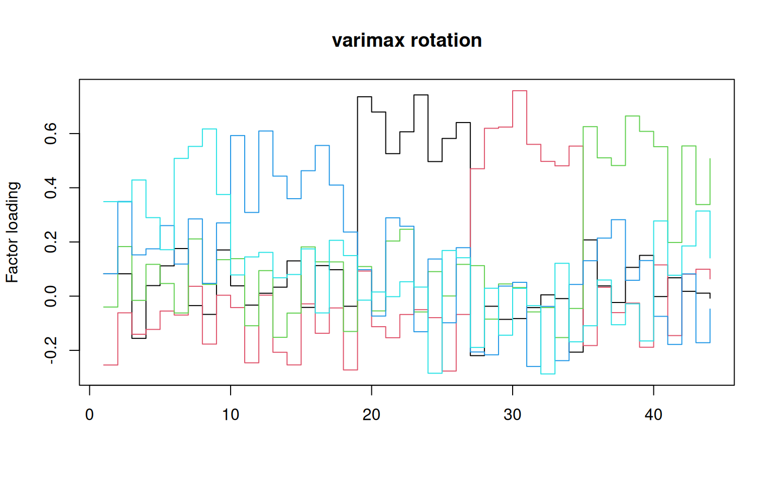
## fairly similar:
matplot(promax(loadings(f2))$loadings, type = "s", lty = 1, main = "promax rotation",
    ylab = "Factor loading")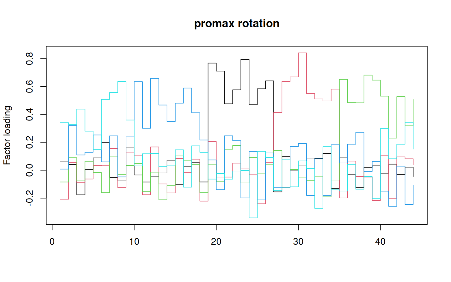
# matplot(oblimin(loadings(f2))$loadings,type='s',lty=1,main='oblimin
# rotation',ylab='Factor loading')

matplot(simplimax(loadings(f2))$loadings, type = "s", lty = 1, main = "simplimax rotation",
    ylab = "Factor loading")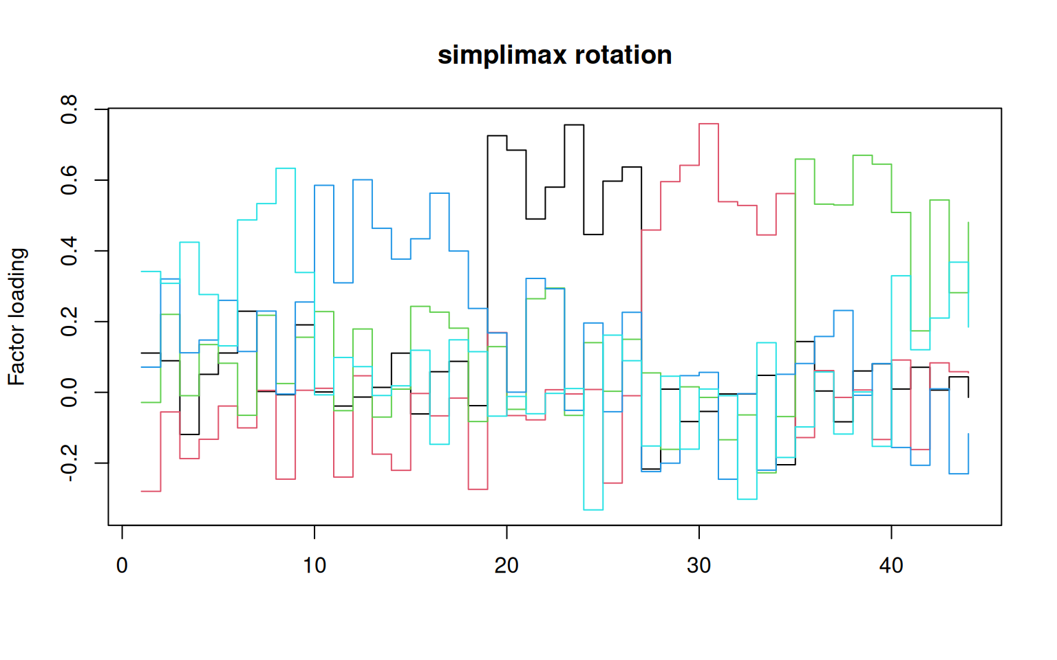
matplot(oblimin(loadings(f2))$loadings, type = "s", lty = 1, main = "oblimin rotation",
    ylab = "Factor loading")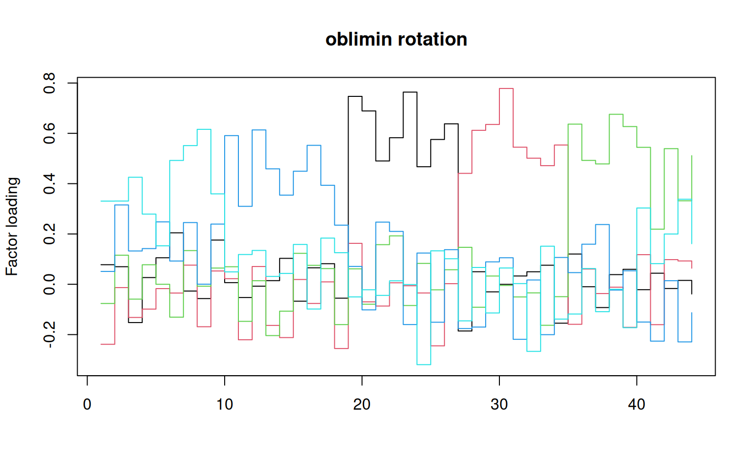
matplot(varimin(loadings(f2))$loadings, type = "s", lty = 1, main = "varimin rotation",
    ylab = "Factor loading")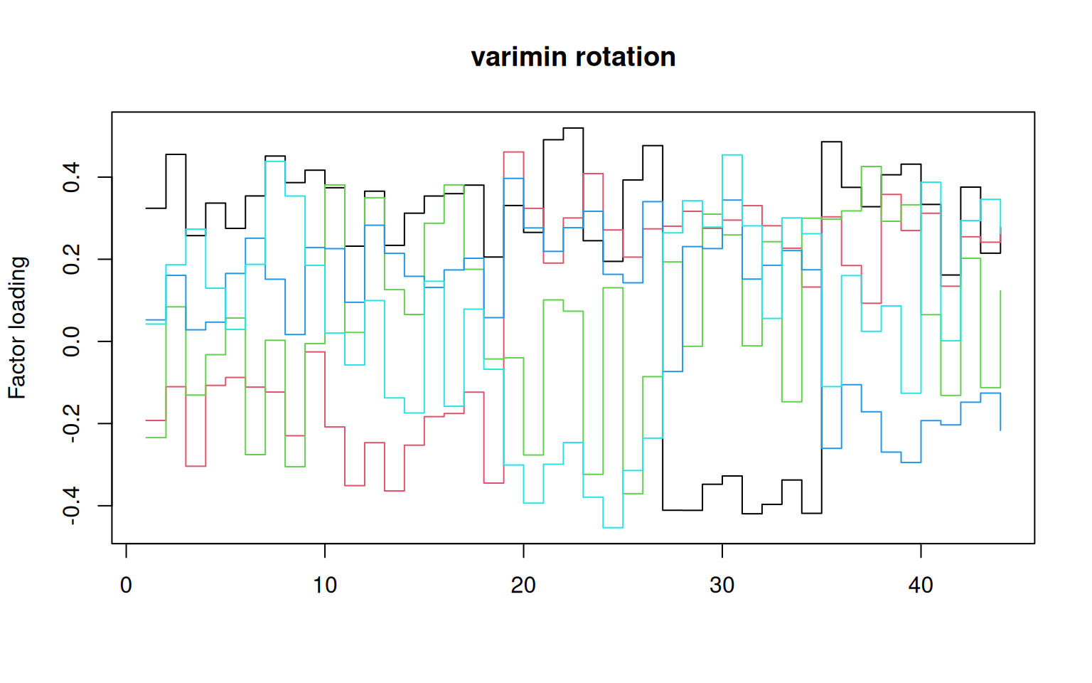
matplot(varimax(loadings(pca)[, 1:5])$loadings, type = "s", lty = 1, main = "varimax rotation on PCA",
    ylab = "Factor loading")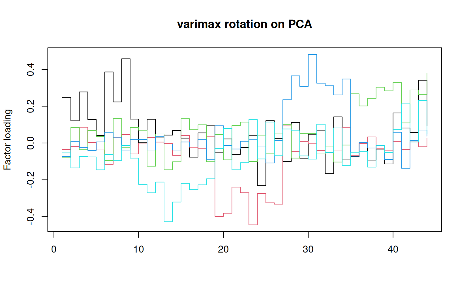
Oblique rotations
If you use an oblique rotation, that means your factors are allowed to be correlated. Here is the full output of an oblique rotation (the oblimin):
Oblique rotation method Oblimin Quartimin converged.
Loadings:
          ML2      ML3       ML4       ML1      ML5
A1   0.077792 -0.23858 -7.63e-02  0.051032  0.33072
A2   0.069772 -0.01312  1.16e-01  0.315380  0.33088
A3  -0.152205 -0.13186 -5.90e-02  0.132431  0.42540
A4   0.026625 -0.09872  7.76e-02  0.141818  0.27891
A5   0.105436 -0.01721 -2.08e-05  0.248122  0.15284
A6   0.204566 -0.03480 -1.31e-01  0.092521  0.49229
A7  -0.026877  0.07607  1.34e-01  0.245298  0.55135
A8  -0.056847 -0.16881 -7.57e-03  0.000358  0.61589
A9   0.175793  0.05282  6.45e-02  0.239280  0.35933
C10  0.006554  0.02231  6.97e-02  0.590989  0.04922
C11 -0.052645 -0.22064 -1.47e-01  0.309812  0.11829
C12 -0.007519  0.07060  1.41e-02  0.613554  0.13442
C13  0.014447 -0.16356 -2.04e-01  0.458906  0.03127
C14  0.102986 -0.21189 -1.07e-01  0.354427  0.04308
C15 -0.067266  0.01906  1.23e-01  0.449388  0.15831
 [ reached getOption("max.print") -- omitted 29 rows ]

                 ML2   ML3   ML4   ML1   ML5
SS loadings    3.522 3.351 3.173 3.028 2.418
Proportion Var 0.080 0.076 0.072 0.069 0.055
Cumulative Var 0.080 0.156 0.228 0.297 0.352

Phi:
        ML2     ML3     ML4    ML1     ML5
ML2  1.0000 -0.1931  0.1603  0.113  0.0184
ML3 -0.1931  1.0000 -0.0149 -0.179 -0.0729
ML4  0.1603 -0.0149  1.0000  0.230  0.0818
ML1  0.1135 -0.1794  0.2296  1.000  0.1240
ML5  0.0184 -0.0729  0.0818  0.124  1.0000
Here, no factors are correlated more than around .2 (see the Phi matrix) which is a constraint in the oblique rotation. The oblique rotations/transformations will sacrifice orthogonality a little in order to maximize another property, usually something about the shared variance of the items that load highly on a factor.
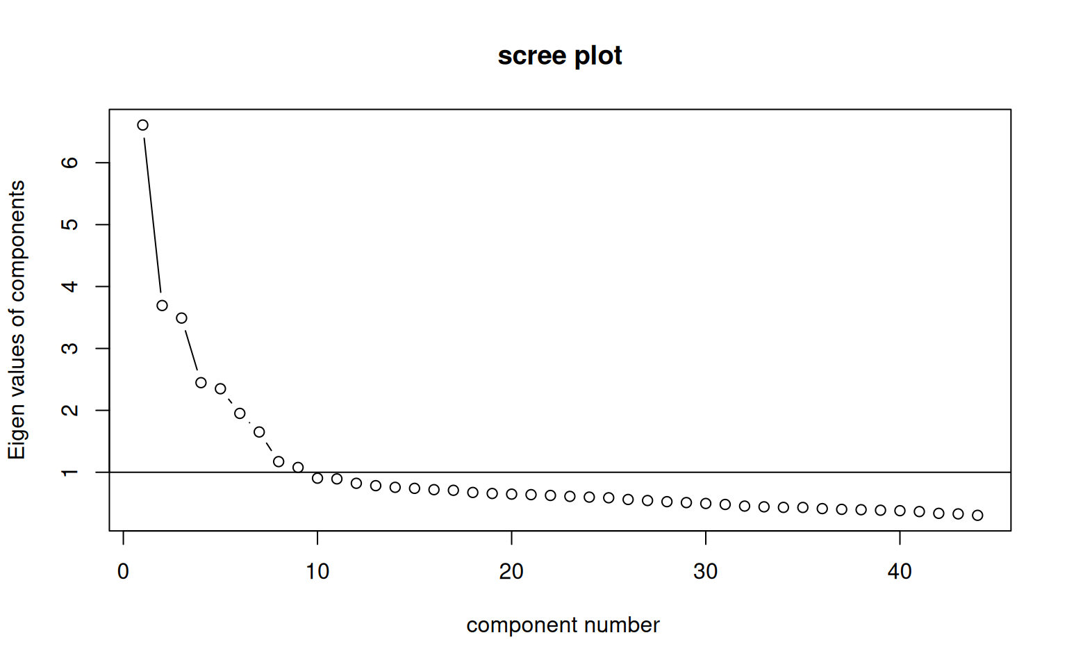
Choosing the right number of factors and evaluating goodness of fit
Like all of the methods we have used, it is tough to know how many factors there are. One approach is to use pca to identify how many factors to use (looking at the scree plot and eigen decomposition). Then do a factor analysis to pick a model with that many dimensions. You can also use the goodness-of-fit statistics reported in the model. Many times, the challenge is that in order to get a model whose goodness-of-fit is large enough to satisfy the basic advice, you need to add more factors than are really interpretable.
Several statistics are available for evaluating goodness of fit, and these can be used to assess the number of factors as well. Detailed tutorials are available at http://davidakenny.net/cm/fit.htm .
Many of the statistics are output from the factor analysis directly, but it may be convenient to use the VSS on the correlation matrix.
Factor analysis with Call: fa(r = bytype, nfactors = 5)

Test of the hypothesis that 5 factors are sufficient.
The degrees of freedom for the model is 736  and the objective function was  3.2
The number of observations was  1017  with Chi Square =  3193.66  with prob <  4.9e-302

The root mean square of the residuals (RMSA) is  0.05
The df corrected root mean square of the residuals is  0.05

Tucker Lewis Index of factoring reliability =  0.762
RMSEA index =  0.057  and the 10 % confidence intervals are  0.055 0.059
BIC =  -1902.86
 With factor correlations of
      MR3   MR4  MR2   MR1   MR5
MR3  1.00 -0.19 0.16  0.13  0.02
MR4 -0.19  1.00 0.00 -0.20 -0.08
MR2  0.16  0.00 1.00  0.23  0.08
MR1  0.13 -0.20 0.23  1.00  0.14
MR5  0.02 -0.08 0.08  0.14  1.00
Factor analysis with Call: fa(r = bytype, nfactors = 8)

Test of the hypothesis that 8 factors are sufficient.
The degrees of freedom for the model is 622  and the objective function was  1.35
The number of observations was  1017  with Chi Square =  1342.04  with prob <  6.3e-55

The root mean square of the residuals (RMSA) is  0.02
The df corrected root mean square of the residuals is  0.03

Tucker Lewis Index of factoring reliability =  0.917
RMSEA index =  0.034  and the 10 % confidence intervals are  0.031 0.036
BIC =  -2965.07
 With factor correlations of
      MR3   MR4   MR2   MR6   MR5   MR8   MR7   MR1
MR3  1.00 -0.18  0.16  0.12 -0.03  0.01  0.06  0.13
MR4 -0.18  1.00 -0.09 -0.30 -0.10 -0.09 -0.05 -0.12
MR2  0.16 -0.09  1.00 -0.04  0.01  0.20  0.20  0.11
MR6  0.12 -0.30 -0.04  1.00  0.10  0.18  0.03  0.02
MR5 -0.03 -0.10  0.01  0.10  1.00 -0.01  0.17  0.06
MR8  0.01 -0.09  0.20  0.18 -0.01  1.00  0.22  0.28
MR7  0.06 -0.05  0.20  0.03  0.17  0.22  1.00  0.08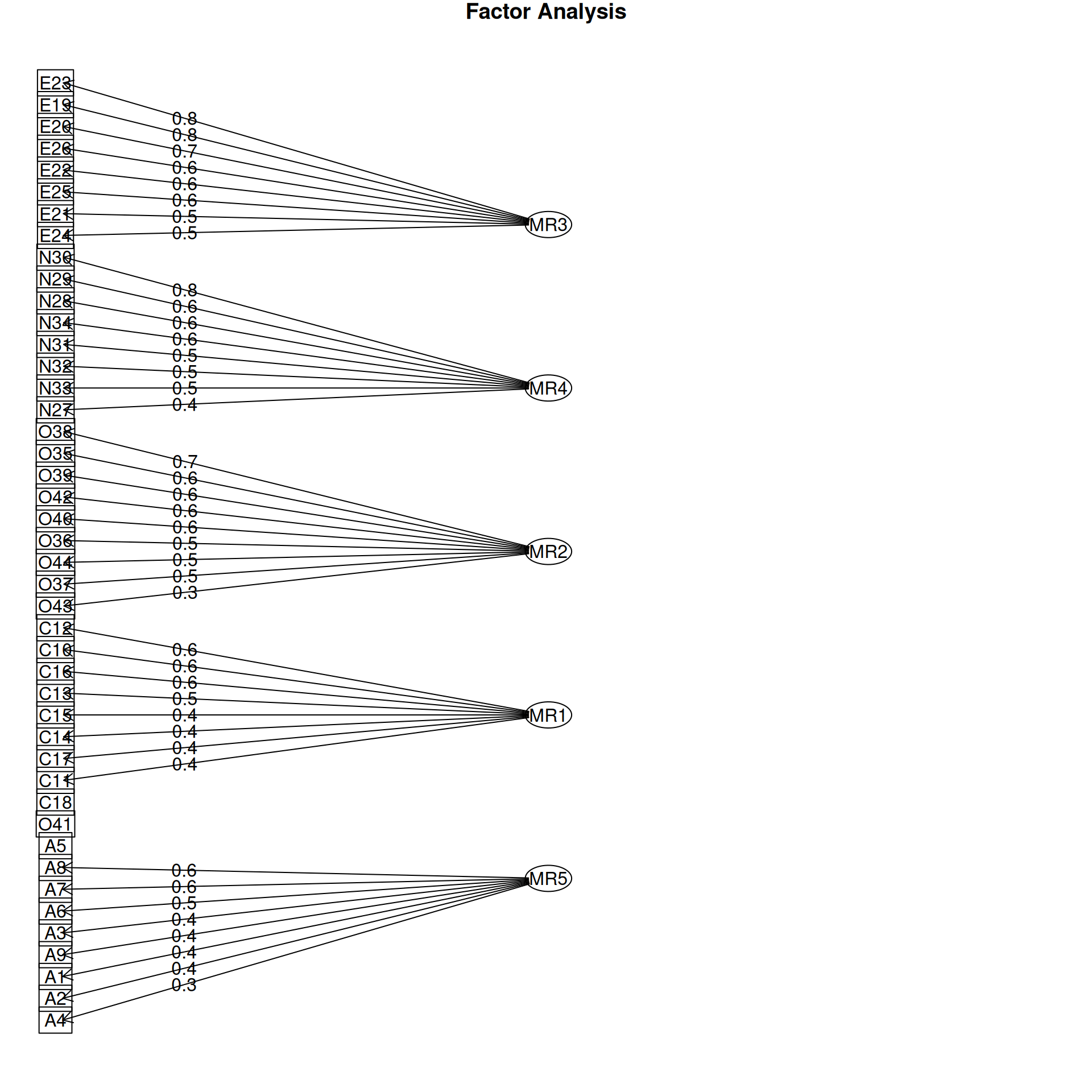
MR1 0.13 -0.12 0.11 0.02 0.06 0.28 0.08 1.00Factor Analysis using method = minres
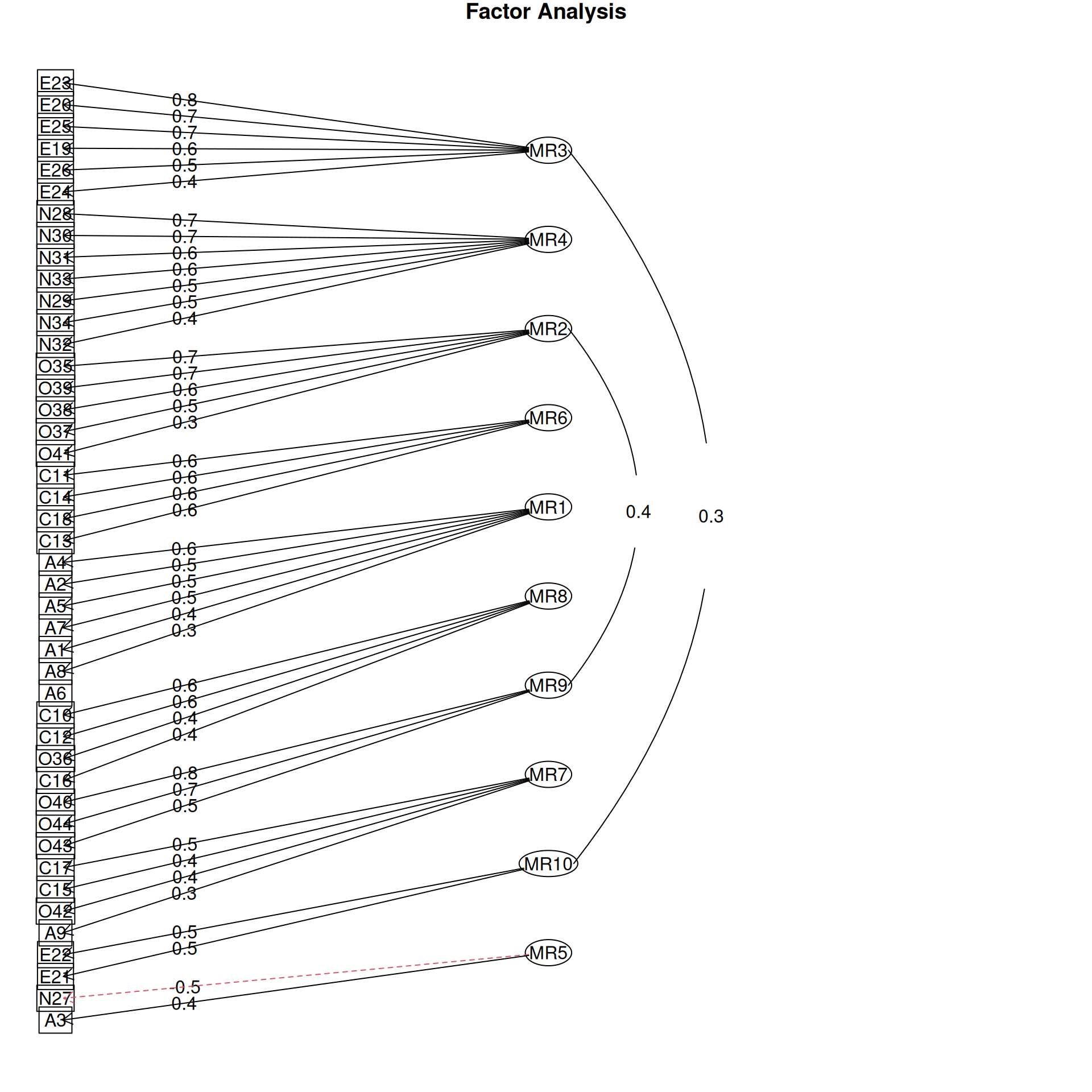
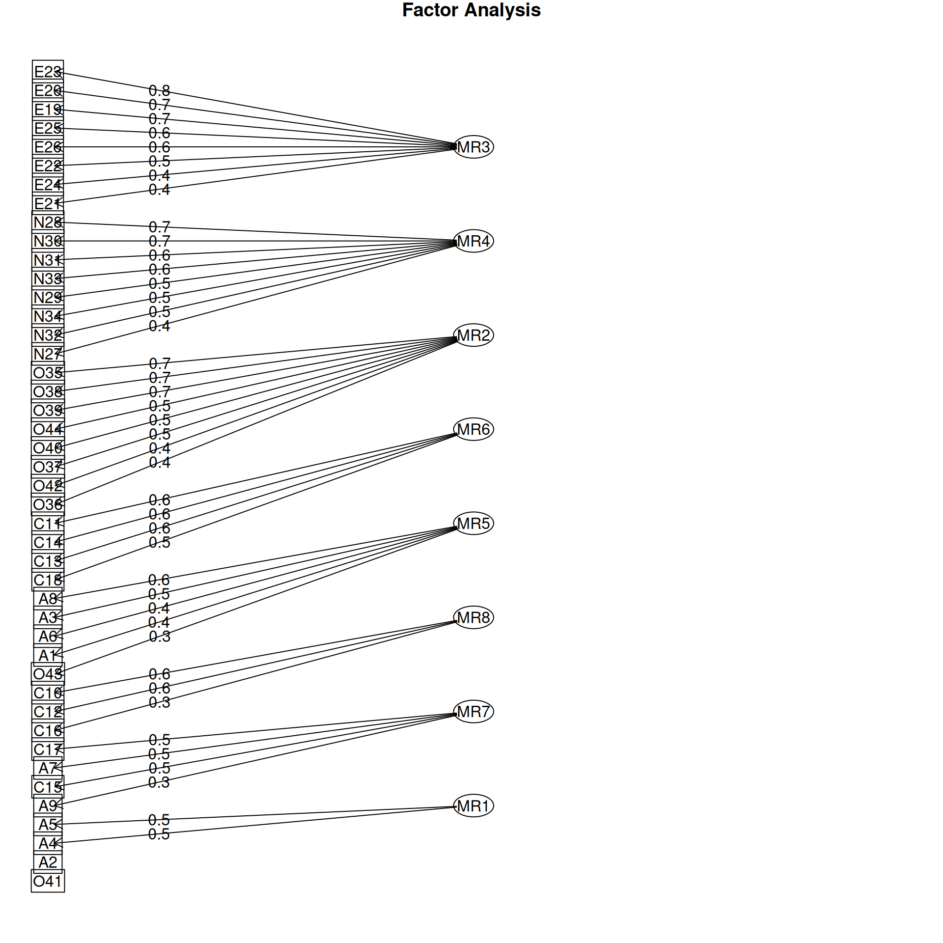
Call: fa(r = bytype, nfactors = 10)
Standardized loadings (pattern matrix) based upon correlation matrix
MR3 MR4 MR2 MR6 MR1 MR8 MR9 MR7 MR10 MR5 h2 u2 com
A1 0.04 -0.06 0.01 0.21 0.41 -0.10 0.02 -0.18 0.04 0.17 0.34 0.66 2.6
A2 0.08 -0.04 0.06 0.02 0.51 0.24 0.02 0.02 -0.07 -0.04 0.39 0.61 1.6
A3 -0.10 0.02 -0.03 0.13 0.28 0.17 0.04 -0.13 -0.12 0.37 0.37 0.63 3.5
A4 -0.06 -0.11 0.07 -0.07 0.61 -0.03 -0.03 -0.07 0.07 -0.02 0.40 0.60 1.2
A5 -0.04 -0.07 0.00 0.00 0.48 -0.01 -0.04 0.00 0.20 -0.14 0.30 0.70 1.6
[ reached 'max' / getOption("max.print") -- omitted 39 rows ]
MR3 MR4 MR2 MR6 MR1 MR8 MR9 MR7 MR10 MR5
SS loadings 2.95 2.83 2.43 2.11 2.02 1.83 1.66 1.49 1.39 1.19
Proportion Var 0.07 0.06 0.06 0.05 0.05 0.04 0.04 0.03 0.03 0.03
Cumulative Var 0.07 0.13 0.19 0.23 0.28 0.32 0.36 0.39 0.43 0.45
Proportion Explained 0.15 0.14 0.12 0.11 0.10 0.09 0.08 0.07 0.07 0.06
Cumulative Proportion 0.15 0.29 0.41 0.52 0.62 0.71 0.80 0.87 0.94 1.00
With factor correlations of
MR3 MR4 MR2 MR6 MR1 MR8 MR9 MR7 MR10 MR5
MR3 1.00 -0.15 0.18 0.10 0.03 -0.06 0.02 0.07 0.32 0.11
MR4 -0.15 1.00 -0.18 -0.27 -0.13 -0.04 0.11 -0.12 -0.10 -0.18
MR2 0.18 -0.18 1.00 0.00 0.08 0.21 0.38 0.09 0.17 -0.05
MR6 0.10 -0.27 0.00 1.00 0.11 0.15 -0.08 0.08 0.00 0.19
MR1 0.03 -0.13 0.08 0.11 1.00 0.21 0.18 0.16 0.17 0.29
MR8 -0.06 -0.04 0.21 0.15 0.21 1.00 0.10 0.21 0.22 -0.04
MR9 0.02 0.11 0.38 -0.08 0.18 0.10 1.00 0.24 -0.06 0.07
[ reached getOption("max.print") -- omitted 3 rows ]
Mean item complexity = 2.2
Test of the hypothesis that 10 factors are sufficient.
df null model = 946 with the objective function = 14.28 with Chi Square = 14284.11
df of the model are 551 and the objective function was 0.98
The root mean square of the residuals (RMSR) is 0.02
The df corrected root mean square of the residuals is 0.02
The harmonic n.obs is 1017 with the empirical chi square 602.99 with prob < 0.062
The total n.obs was 1017 with Likelihood Chi Square = 970.8 with prob < 1.3e-25
Tucker Lewis Index of factoring reliability = 0.946
RMSEA index = 0.027 and the 90 % confidence intervals are 0.025 0.03
BIC = -2844.66
Fit based upon off diagonal values = 0.99
Measures of factor score adequacy
MR3 MR4 MR2 MR6 MR1 MR8
Correlation of (regression) scores with factors 0.93 0.92 0.91 0.88 0.87 0.86
Multiple R square of scores with factors 0.86 0.84 0.82 0.77 0.76 0.75
Minimum correlation of possible factor scores 0.73 0.69 0.64 0.55 0.52 0.49
MR9 MR7 MR10 MR5
Correlation of (regression) scores with factors 0.88 0.84 0.85 0.81
Multiple R square of scores with factors 0.77 0.71 0.71 0.66
Minimum correlation of possible factor scores 0.55 0.42 0.43 0.31
Factor analysis with Call: fa(r = bytype, nfactors = 10)

Test of the hypothesis that 10 factors are sufficient.
The degrees of freedom for the model is 551  and the objective function was  0.98
The number of observations was  1017  with Chi Square =  970.8  with prob <  1.3e-25

The root mean square of the residuals (RMSA) is  0.02
The df corrected root mean square of the residuals is  0.02

Tucker Lewis Index of factoring reliability =  0.946
RMSEA index =  0.027  and the 10 % confidence intervals are  0.025 0.03
BIC =  -2844.66
 With factor correlations of
       MR3   MR4   MR2   MR6   MR1   MR8   MR9   MR7  MR10   MR5
MR3   1.00 -0.15  0.18  0.10  0.03 -0.06  0.02  0.07  0.32  0.11
MR4  -0.15  1.00 -0.18 -0.27 -0.13 -0.04  0.11 -0.12 -0.10 -0.18
MR2   0.18 -0.18  1.00  0.00  0.08  0.21  0.38  0.09  0.17 -0.05
MR6   0.10 -0.27  0.00  1.00  0.11  0.15 -0.08  0.08  0.00  0.19
MR1   0.03 -0.13  0.08  0.11  1.00  0.21  0.18  0.16  0.17  0.29
MR8  -0.06 -0.04  0.21  0.15  0.21  1.00  0.10  0.21  0.22 -0.04
MR9   0.02  0.11  0.38 -0.08  0.18  0.10  1.00  0.24 -0.06  0.07
[ reached getOption("max.print") -- omitted 3 rows ][1] -1902.859 -2965.069 -2844.663Here, the 8-factor solution has the best BIC, the 4-factor solution has high RMSEA and low TLI, so it is probably not good.
Determining the number of factors
There are a number of approaches to picking the number of factors. As suggested by the VSS help file: > 1. Extracting factors until the chi square of the residual matrix is not significant. > 2. Extracting factors until the change in chi square from factor n to factor n+1 is not significant. > 3. Extracting factors until the eigen values of the real data are less than the corresponding eigen values of a random data set of the same size (parallel analysis) using fa.parallel. > 4. Plotting the magnitude of the successive eigen values and applying the scree test (a sudden drop in eigen values analogous to the change in slope seen when scrambling up the talus slope of a mountain and approaching the rock face. > 5. Extracting principal components until the eigen value < 1, and use that many factors. > 6. Extracting factors as long as they are interpetable. > 7. Using the Very Simple Structure Criterion (VSS). > 8. Using Wayne Velicer’s Minimum Average Partial (MAP) criterion.
The VSS function will display many of these criteria in a table. You can use any of these criteria, and we will look at many of them more specifically below. The output includes:
dof: degrees of freedom (if using FA)
chisq: chi square (from the factor analysis output (if using FA)
prob: probability of residual matrix > 0 (if using FA)
sqresid: squared residual correlations
RMSEA: the RMSEA for each number of factors
BIC: the BIC for each number of factors
eChiSq: the empirically found chi square
eRMS: Empirically found mean residual
eCRMS: Empirically found mean residual corrected for df
eBIC: The empirically found BIC based upon the eChiSq
fit: factor fit of the complete model
cfit.1: VSS fit of complexity 1
cfit.2: VSS fit of complexity 2
cfit.8: VSS fit of complexity 8
cresidiual.1: sum squared residual correlations for complexity 1
: sum squared residual correlations for complexity 2 ..8
Running VSS requires giving it the raw correlation matrix:
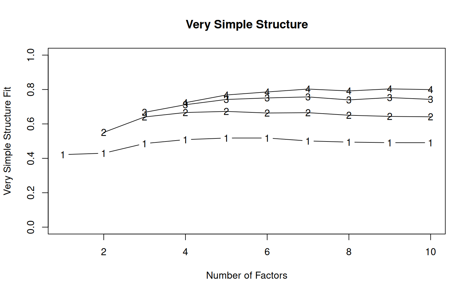
Very Simple Structure
Call: vss(x = x, n = n, rotate = rotate, diagonal = diagonal, fm = fm,
    n.obs = n.obs, plot = plot, title = title, use = use, cor = cor)
VSS complexity 1 achieves a maximimum of 0.52  with  6  factors
VSS complexity 2 achieves a maximimum of 0.67  with  5  factors

The Velicer MAP achieves a minimum of 0.01  with  7  factors
BIC achieves a minimum of  -2977.51  with  8  factors
Sample Size adjusted BIC achieves a minimum of  -1101.97  with  10  factors

Statistics by number of factors
  vss1 vss2   map dof chisq prob sqresid  fit RMSEA   BIC SABIC complex eChisq
1 0.42 0.00 0.019 902  9845    0      59 0.42 0.100  3614  6479     1.0  25559
2 0.43 0.55 0.016 859  7801    0      46 0.55 0.090  1868  4596     1.4  17254
3 0.49 0.64 0.013 817  5617    0      34 0.67 0.077   -26  2568     1.5   9725
4 0.51 0.67 0.011 776  4260    0      28 0.72 0.067 -1101  1364     1.6   6604
   SRMR eCRMS  eBIC
1 0.116 0.119 19328
2 0.095 0.100 11320
3 0.072 0.077  4082
4 0.059 0.065  1244
 [ reached 'max' / getOption("max.print") -- omitted 6 rows ]
These parallel lines are VSS statistics for reconstituting the correlation matrix with different numbers of simple factors, with the number indicating the complexity. VSS1 picks the largest value for each factor, VSS2 shows the two largest, etc. These two are shown numerically, and complexity 3 and 4 are also shown in the graph visually. The help suggests that these will peak at the optimal number of factors. Here, the output suggests the optimal is between 5 and 8, depending on your criterion.
Summary of goodness-of-fit statistics.
VSS
VSS scores tend to peak at a number of factors that is ‘most interpretable’. They compare the fit of the simplified model to the original correlations.
RMSEA
RMSEA score is a measure of root mean square error residuals. It says how far off you are, on average, when you compare the predicted correlation matrix and the actual one. Here, for 5 factors, it is .058, which is reasonably ‘good’, but not great (a RMSEA of .01 would be great). For 10 factors, it gets down to .028–but at what cost?
A RMSEA of .05 means that when you try to estimate the correlation matrix, each error is off by about .05.
TLI
TLI (Tucker-Lewis Index) is based on comparing expected versus observed chi-squared tests, penalizing by the size of the model. Here, it is .764 for 5 groups and .95 for 10 groups. A value of .9 is considered marginal, .95+ is good. So, 5 groups would be considered inadequate.
BIC and AIC
BIC is a relative measure, which combines goodness of fit in its likelihood with model complexity. Smaller or more negative scores are better. Here, BIC for 5-factor is -1919, and for 10-factor it is -2854.69. We need to be careful about interpreting BIC because sometimes functions report negative BIC. In this case, we are looking for the minimum BIC score, which occurs at 8 factors.
MAP: Velicer’s Minimal Average Partial
This will tend to minimize for the ‘best’ model.
Interpretability
More often than not, researchers rely on notions of interpretability to guide exploratory factor analysis. The statistics may tell you a ten-factor solution is needed, but you may only be able to interpret three. Ultimately, the goal of FA is usually scientific inference, and if the factor is not helping you understand anything, it might not be helpful to use.
Assessing general factors with the omega function
In intelligence research, factor analysis has often revealed a general intelligence element g that is general across all skills.
library(psych)
library(lavaan)

dat <- HolzingerSwineford1939[, 7:15]
colnames(dat) <- c("vis", "cubes", "lozenges", "pcomp", "scomp", "meaning", "addition",
    "counting", "letters")
VSS(cor(dat), n = 5)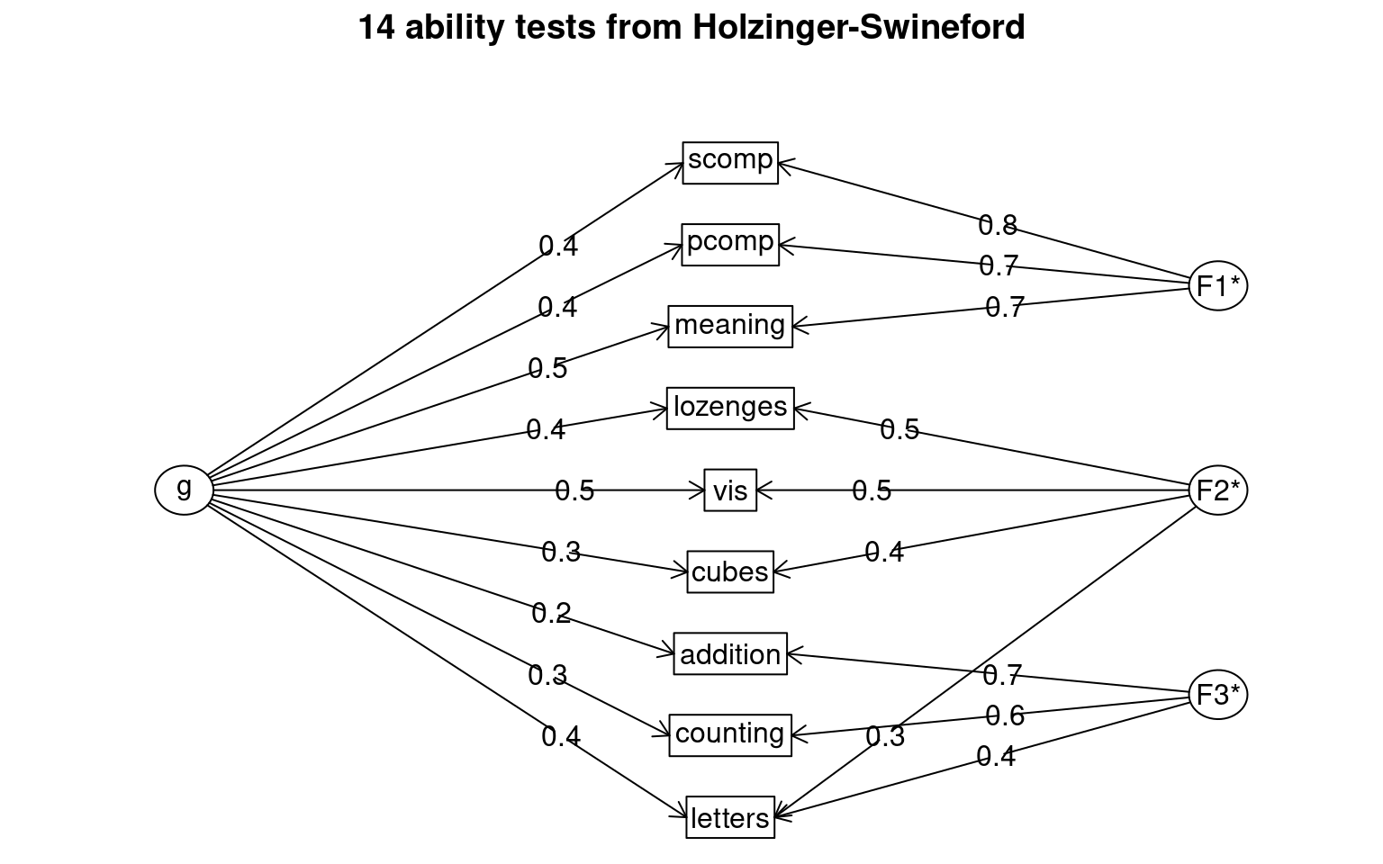
Very Simple Structure
Call: vss(x = x, n = n, rotate = rotate, diagonal = diagonal, fm = fm,
    n.obs = n.obs, plot = plot, title = title, use = use, cor = cor)
VSS complexity 1 achieves a maximimum of 0.7  with  3  factors
VSS complexity 2 achieves a maximimum of 0.85  with  3  factors

The Velicer MAP achieves a minimum of 0.06  with  2  factors
BIC achieves a minimum of  -22.87  with  4  factors
Sample Size adjusted BIC achieves a minimum of  -3.81  with  4  factors

Statistics by number of factors
  vss1 vss2   map dof chisq     prob sqresid  fit RMSEA    BIC  SABIC complex
1 0.61 0.00 0.080  27  1206 4.8e-237     6.4 0.61 0.209 1019.3 1105.1     1.0
2 0.65 0.76 0.063  19   436  1.7e-80     3.9 0.76 0.148  304.3  364.7     1.2
3 0.70 0.85 0.068  12    76  2.2e-11     2.1 0.87 0.073   -6.7   31.4     1.3
4 0.66 0.84 0.120   6    19  4.9e-03     1.8 0.89 0.046  -22.9   -3.8     1.4
  eChisq   SRMR eCRMS eBIC
1 1557.0 0.1471 0.170 1370
2  511.9 0.0843 0.116  381
3   26.1 0.0191 0.033  -57
4    5.5 0.0088 0.021  -36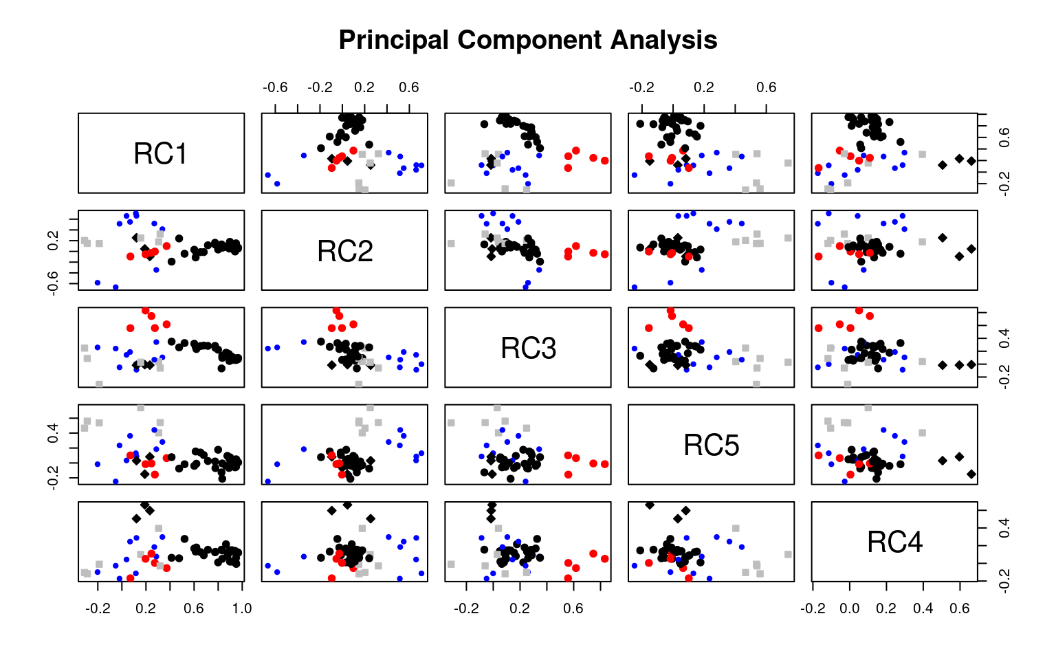
[ reached 'max' / getOption("max.print") -- omitted 1 rows ]Principal Components Analysis
Call: principal(r = r, nfactors = nfactors, residuals = residuals,
rotate = rotate, n.obs = n.obs, covar = covar, scores = scores,
missing = missing, impute = impute, oblique.scores = oblique.scores,
method = method, use = use, cor = cor, correct = 0.5, weight = NULL)
Standardized loadings (pattern matrix) based upon correlation matrix
RC1 RC3 RC2 h2 u2 com
vis 0.32 0.67 0.17 0.59 0.41 1.6
cubes 0.08 0.73 -0.10 0.55 0.45 1.1
lozenges 0.02 0.78 0.15 0.63 0.37 1.1
pcomp 0.89 0.12 0.09 0.81 0.19 1.1
scomp 0.90 0.06 0.08 0.82 0.18 1.0
meaning 0.87 0.18 0.08 0.79 0.21 1.1
addition 0.10 -0.15 0.83 0.72 0.28 1.1
counting 0.04 0.14 0.82 0.69 0.31 1.1
letters 0.13 0.44 0.64 0.61 0.39 1.9
RC1 RC3 RC2
SS loadings 2.50 1.87 1.85
Proportion Var 0.28 0.21 0.21
Cumulative Var 0.28 0.49 0.69
Proportion Explained 0.40 0.30 0.30
Cumulative Proportion 0.40 0.70 1.00
Mean item complexity = 1.2
Test of the hypothesis that 3 components are sufficient.
The root mean square of the residuals (RMSR) is 0.08
Fit based upon off diagonal values = 0.93The default 3D pca of this data set shows three main factors with strong structure. The uniqueness suggests there is substantial error in each dimension not captured otherwise. How does FA do? Can we estimate a more general factor shared across all dimensions? Let’s try an EFA with both 3 and 4 dimensions. I will use varimax rotation to enforce orthogonal factors.
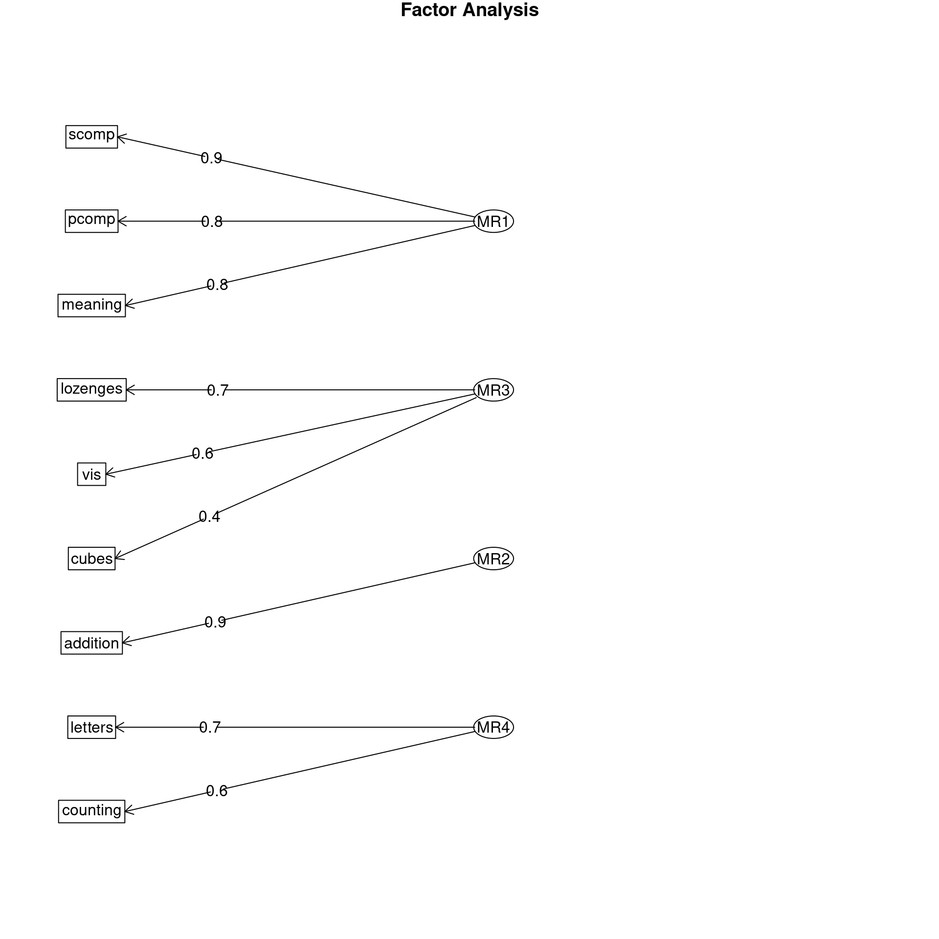
Factor Analysis using method =  minres
Call: fa(r = dat, nfactors = 3, rotate = "varimax")
Standardized loadings (pattern matrix) based upon correlation matrix
          MR1   MR3   MR2   h2   u2 com
vis      0.28  0.61  0.15 0.48 0.52 1.5
cubes    0.10  0.49 -0.03 0.26 0.74 1.1
lozenges 0.04  0.66  0.13 0.45 0.55 1.1
pcomp    0.83  0.16  0.10 0.73 0.27 1.1
scomp    0.86  0.09  0.09 0.75 0.25 1.0
meaning  0.80  0.21  0.09 0.69 0.31 1.2
addition 0.09 -0.08  0.71 0.52 0.48 1.1
counting 0.05  0.17  0.70 0.52 0.48 1.1
letters  0.13  0.41  0.52 0.46 0.54 2.0

                       MR1  MR3  MR2
SS loadings           2.19 1.34 1.33
Proportion Var        0.24 0.15 0.15
Cumulative Var        0.24 0.39 0.54
Proportion Explained  0.45 0.28 0.27
Cumulative Proportion 0.45 0.73 1.00

Mean item complexity =  1.3
Test of the hypothesis that 3 factors are sufficient.

df null model =  36  with the objective function =  3.05 with Chi Square =  904.1
df of  the model are 12  and the objective function was  0.08

The root mean square of the residuals (RMSR) is  0.02
The df corrected root mean square of the residuals is  0.03

The harmonic n.obs is  301 with the empirical chi square  7.87  with prob <  0.8
The total n.obs was  301  with Likelihood Chi Square =  22.56  with prob <  0.032

Tucker Lewis Index of factoring reliability =  0.963
RMSEA index =  0.054  and the 90 % confidence intervals are  0.016 0.088
BIC =  -45.93
Fit based upon off diagonal values = 1
Measures of factor score adequacy
                                                   MR1  MR3  MR2
Correlation of (regression) scores with factors   0.93 0.81 0.84
Multiple R square of scores with factors          0.87 0.66 0.70
Minimum correlation of possible factor scores 0.74 0.32 0.41Factor Analysis using method = minres
Call: fa(r = dat, nfactors = 4, rotate = "varimax")
Standardized loadings (pattern matrix) based upon correlation matrix
MR1 MR3 MR2 MR4 h2 u2 com
vis 0.29 0.56 0.00 0.24 0.45 0.5464 1.9
cubes 0.11 0.45 -0.09 0.09 0.23 0.7702 1.3
lozenges 0.03 0.73 0.09 0.11 0.55 0.4460 1.1
pcomp 0.83 0.18 0.11 0.03 0.74 0.2602 1.1
scomp 0.87 0.04 -0.03 0.16 0.79 0.2132 1.1
meaning 0.80 0.21 0.05 0.07 0.69 0.3133 1.2
addition 0.09 -0.07 0.93 0.36 1.00 0.0035 1.3
counting 0.06 0.13 0.32 0.55 0.42 0.5756 1.8
letters 0.13 0.33 0.13 0.65 0.57 0.4321 1.7
MR1 MR3 MR2 MR4
SS loadings 2.21 1.26 1.01 0.97
Proportion Var 0.25 0.14 0.11 0.11
Cumulative Var 0.25 0.39 0.50 0.60
Proportion Explained 0.41 0.23 0.18 0.18
Cumulative Proportion 0.41 0.64 0.82 1.00
Mean item complexity = 1.4
Test of the hypothesis that 4 factors are sufficient.
df null model = 36 with the objective function = 3.05 with Chi Square = 904.1
df of the model are 6 and the objective function was 0.02
The root mean square of the residuals (RMSR) is 0.01
The df corrected root mean square of the residuals is 0.02
The harmonic n.obs is 301 with the empirical chi square 1.66 with prob < 0.95
The total n.obs was 301 with Likelihood Chi Square = 5.49 with prob < 0.48
Tucker Lewis Index of factoring reliability = 1.004
RMSEA index = 0 and the 90 % confidence intervals are 0 0.071
BIC = -28.75
Fit based upon off diagonal values = 1
Measures of factor score adequacy
MR1 MR3 MR2 MR4
Correlation of (regression) scores with factors 0.94 0.82 0.96 0.74
Multiple R square of scores with factors 0.88 0.67 0.92 0.55
Minimum correlation of possible factor scores 0.76 0.34 0.84 0.10The FA with 3 finds a slightly different model, with letters fitting into visual more than speed–this was a task discriminating upper and lowercase letters, so maybe there is some truth to that. The factor analysis with 4 dimensions separates that into its own dimension. None of these capture a single common model, in order to estimate a ‘g’ factor.
A traditional version of the bifactor model is available in the omega
function in psych, which fits a general factor and then an
EFA on the residuals, and comparing the difference between these models.
This is more like EFA with a specific structure. The model implements a
factor analysis that fits one common factor and then unique
factors–attempting to identify the ‘g’ general factor that is commonly
found in intelligence research. Also, we discussed this model when
examining psychometrics: this is argued to be the best way to identify
whether a single factor exists, and more instructive than measures such
as cohen’s \(\alpha\) or GLB.
14 ability tests from Holzinger-Swineford
Call: omegah(m = m, nfactors = nfactors, fm = fm, key = key, flip = flip,
    digits = digits, title = title, sl = sl, labels = labels,
    plot = plot, n.obs = n.obs, rotate = rotate, Phi = Phi, option = option,
    covar = covar)
Alpha:                 0.76
G.6:                   0.81
Omega Hierarchical:    0.45
Omega H asymptotic:    0.53
Omega Total            0.85

Schmid Leiman Factor loadings greater than  0.2
            g   F1*   F2*   F3*   h2   u2   p2
vis      0.49        0.46       0.48 0.52 0.49
cubes    0.29        0.40       0.26 0.74 0.33
lozenges 0.41        0.53       0.45 0.55 0.37
pcomp    0.45  0.73             0.73 0.27 0.28
scomp    0.42  0.76             0.75 0.25 0.23
meaning  0.46  0.69             0.69 0.31 0.30
addition 0.23              0.67 0.52 0.48 0.10
counting 0.35              0.62 0.52 0.48 0.23
letters  0.45        0.30  0.42 0.46 0.54 0.43

With Sums of squares  of:
   g  F1*  F2*  F3*
1.44 1.62 0.77 1.03

general/max  0.89   max/min =   2.09
mean percent general =  0.31    with sd =  0.12 and cv of  0.38
Explained Common Variance of the general factor =  0.3

The degrees of freedom are 12  and the fit is  0.08
The number of observations was  301  with Chi Square =  22.56  with prob <  0.032
The root mean square of the residuals is  0.02
The df corrected root mean square of the residuals is  0.03
RMSEA index =  0.054  and the 10 % confidence intervals are  0.016 0.088
BIC =  -45.93

Compare this with the adequacy of just a general factor and no group factors
The degrees of freedom for just the general factor are 27  and the fit is  1.75
The number of observations was  301  with Chi Square =  517.02  with prob <  4.7e-92
The root mean square of the residuals is  0.2
The df corrected root mean square of the residuals is  0.23

RMSEA index =  0.246  and the 10 % confidence intervals are  0.228 0.265
BIC =  362.93

Measures of factor score adequacy
                                                  g  F1*   F2*  F3*
Correlation of scores with factors             0.68 0.84  0.67 0.79
Multiple R square of scores with factors       0.46 0.71  0.45 0.62
Minimum correlation of factor score estimates -0.08 0.42 -0.10 0.23

 Total, General and Subset omega for each subset
                                                 g  F1*  F2*  F3*
Omega total for total scores and subscales    0.85 0.89 0.65 0.72
Omega general for total scores and subscales  0.45 0.24 0.27 0.19
Omega group for total scores and subscales    0.35 0.65 0.37 0.53
Notice that the g factor is relatively strong here, and each of three factors load uniquely on a small subset of the other variables, and it also captures this ‘intermediate’ letter test. It also tests this complete model against the single group factor, so if the model fails, it suggests no more than one group is needed–that is, you have a coherent structure or a consensus. Thus, if that test fails, it may be the best approach to estimating a strong structure as an alternative to Cohen’s alpha–providing the first factor is sufficiently good.
We can try the ability.cov data as well using omega. 3 factors looks like it is too many, but a general factor is formed. 28% of the variance is accounted for by the common factor:

Omega
Call: omegah(m = m, nfactors = nfactors, fm = fm, key = key, flip = flip,
    digits = digits, title = title, sl = sl, labels = labels,
    plot = plot, n.obs = n.obs, rotate = rotate, Phi = Phi, option = option,
    covar = covar)
Alpha:                 0.86
G.6:                   0.91
Omega Hierarchical:    0.4
Omega H asymptotic:    0.42
Omega Total            0.96

Schmid Leiman Factor loadings greater than  0.2
           g   F1*   F2*   h2    u2   p2
general 0.60  0.49  0.49 0.84  0.16 0.43
picture 0.47  0.78       0.83  0.17 0.26
blocks  0.53  0.88       1.05 -0.05 0.27
maze    0.34  0.65       0.56  0.44 0.21
reading 0.50        0.87 1.00  0.00 0.25
vocab   0.49        0.82 0.91  0.09 0.26

With Sums of squares  of:
  g F1* F2*
1.5 2.0 1.7

general/max  0.71   max/min =   1.23
mean percent general =  0.28    with sd =  0.08 and cv of  0.27
Explained Common Variance of the general factor =  0.28

The degrees of freedom are 4  and the fit is  19.35
The number of observations was  6  with Chi Square =  16.13  with prob <  0.0029
The root mean square of the residuals is  0.02
The df corrected root mean square of the residuals is  0.05
RMSEA index =  0.687  and the 10 % confidence intervals are  0.408 NA
BIC =  8.96

Compare this with the adequacy of just a general factor and no group factors
The degrees of freedom for just the general factor are 9  and the fit is  25.45
The number of observations was  6  with Chi Square =  38.18  with prob <  1.6e-05
The root mean square of the residuals is  0.4
The df corrected root mean square of the residuals is  0.51

RMSEA index =  0.712  and the 10 % confidence intervals are  0.552 NA
BIC =  22.06

Measures of factor score adequacy
                                                  g  F1*  F2*
Correlation of scores with factors             0.65 0.86 0.88
Multiple R square of scores with factors       0.42 0.74 0.77
Minimum correlation of factor score estimates -0.16 0.49 0.55

 Total, General and Subset omega for each subset
                                                 g  F1*  F2*
Omega total for total scores and subscales    0.96 0.92 0.94
Omega general for total scores and subscales  0.40 0.23 0.33
Omega group for total scores and subscales    0.48 0.69 0.62
Omega
Call: omegah(m = m, nfactors = nfactors, fm = fm, key = key, flip = flip,
    digits = digits, title = title, sl = sl, labels = labels,
    plot = plot, n.obs = n.obs, rotate = rotate, Phi = Phi, option = option,
    covar = covar)
Alpha:                 0.86
G.6:                   0.91
Omega Hierarchical:    0.65
Omega H asymptotic:    0.66
Omega Total            0.99

Schmid Leiman Factor loadings greater than  0.2
           g   F1* F2*   F3*   h2   u2   p2
general 0.71  0.57           0.84 0.16 0.60
picture 0.99                 0.98 0.02 1.01
blocks  0.97            0.23 1.00 0.00 0.95
maze    0.65            0.76 1.00 0.00 0.42
reading 0.20  0.97           1.00 0.00 0.04
vocab   0.20  0.94           0.92 0.08 0.04

With Sums of squares  of:
   g  F1*  F2*  F3*
2.93 2.16 0.00 0.63

general/max  1.36   max/min =   Inf
mean percent general =  0.51    with sd =  0.42 and cv of  0.83
Explained Common Variance of the general factor =  0.51

The degrees of freedom are 0  and the fit is  17.39
The number of observations was  6  with Chi Square =  2.9  with prob <  NA
The root mean square of the residuals is  0
The df corrected root mean square of the residuals is  NA

Compare this with the adequacy of just a general factor and no group factors
The degrees of freedom for just the general factor are 9  and the fit is  23.53
The number of observations was  6  with Chi Square =  35.29  with prob <  5.3e-05
The root mean square of the residuals is  0.32
The df corrected root mean square of the residuals is  0.41

RMSEA index =  0.673  and the 10 % confidence intervals are  0.509 NA
BIC =  19.16

Measures of factor score adequacy
                                                 g  F1* F2*  F3*
Correlation of scores with factors            1.00 1.01   0 1.01
Multiple R square of scores with factors      1.00 1.01   0 1.01
Minimum correlation of factor score estimates 0.99 1.03  -1 1.02

 Total, General and Subset omega for each subset
                                                 g  F1* F2*  F3*
Omega total for total scores and subscales    0.99 0.96  NA 0.99
Omega general for total scores and subscales  0.65 0.41  NA 0.73
Omega group for total scores and subscales    0.33 0.55  NA 0.27
The bifactor model produced by omega includes a general
factor and then multiple additional unique factors. The interpretation
of these is a bit tricky–these might be thought of as the systematic
parts NOT included in the general factor. In this case, what are the
things that general intelligence, reading, and vocabulary share that
aren’t general intelligence? The interpretation is also tricky because
reading and vocab are relatively low in g, but high in F1.
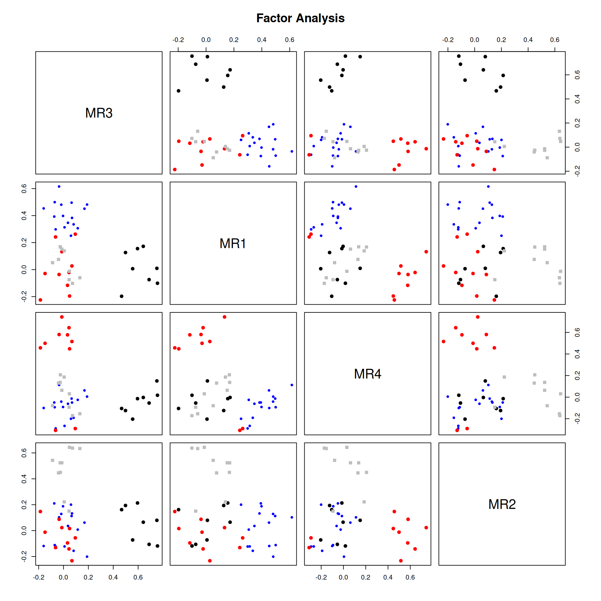
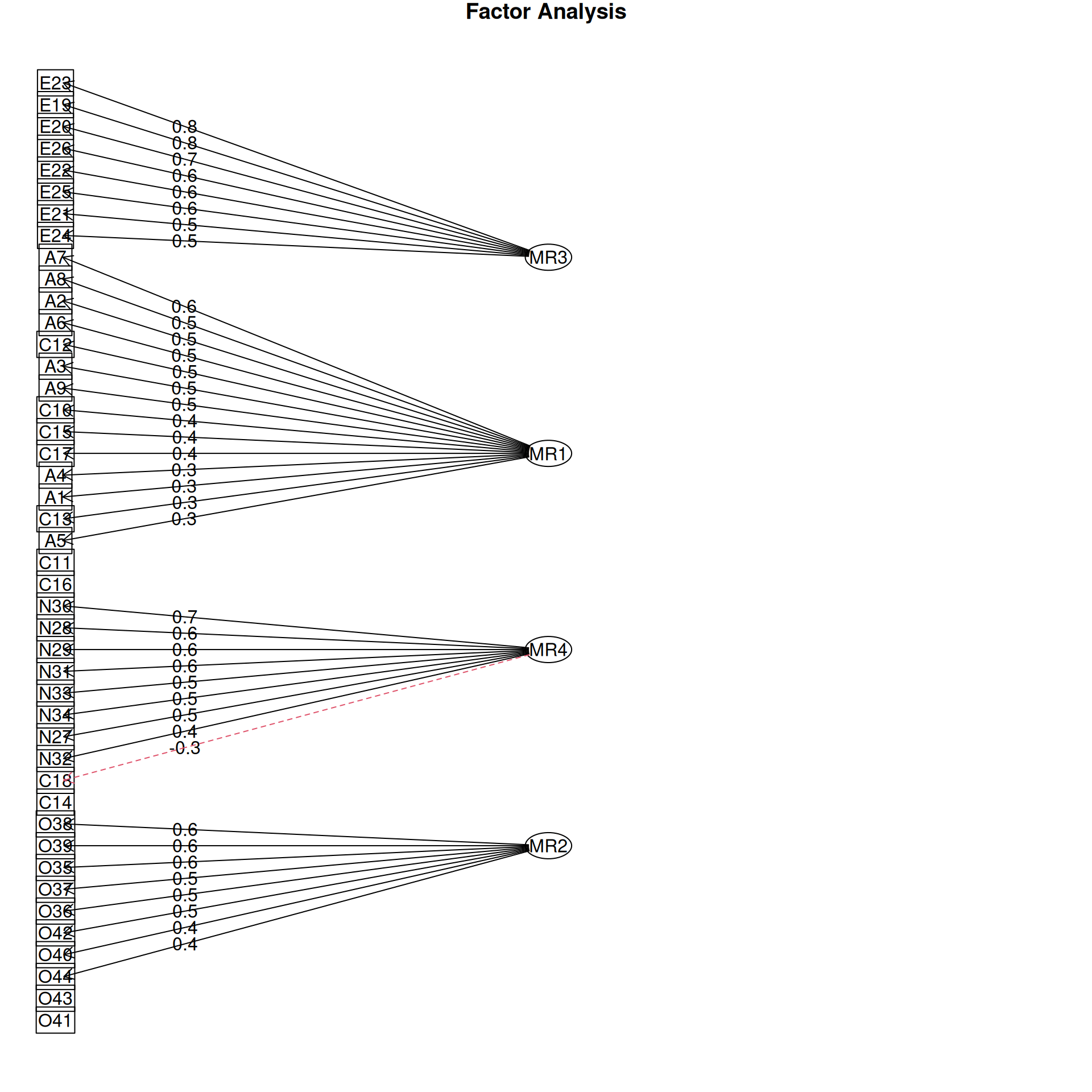
Examining and displaying the models
It is common to display the results in several ways that show the factor structure. if you use the plot method, it will show you the points along each pair of dimensions, with point color-coded by whether they are high or low on each dimension. Looking at some of the FAs:
Example: Michigan House Votes
Use the Michigan house votes to compute a factor analysis. If necessary, determine what to do for ‘impute’, figure out how many factors to use, explore several rotations, and try to identify an interpretable result.
Assessing factors of political issues
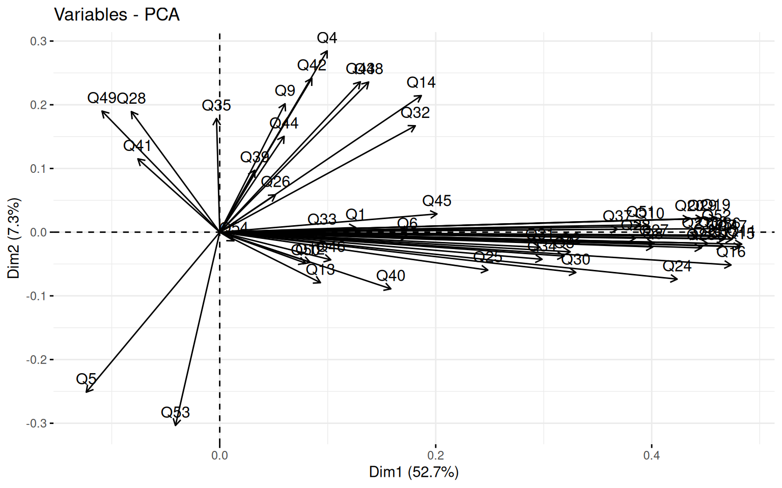
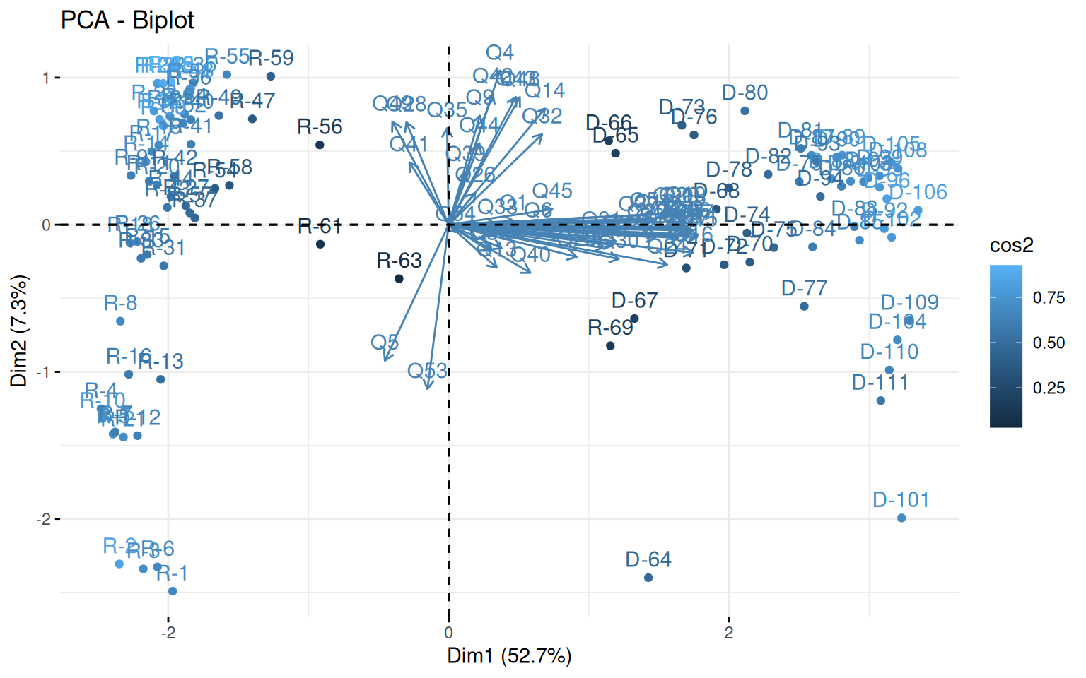
First we can look at a PCA to get an idea of the number of factors that might exist in the data. fvis_pca provides some interesting visualizations:
library(factoextra)
house <- read.csv("mihouse.csv")
votes <- house[, -(1:2)]
rownames(votes) <- paste(house$Party, 1:nrow(house), sep = "-")
pca <- princomp(~., data = votes, scores = T)  #this handles NA values
fviz_screeplot(pca)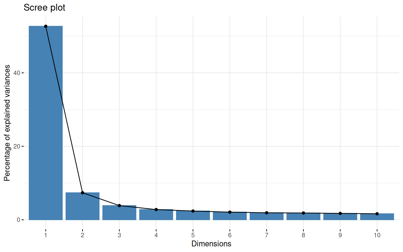
Call:
princomp(formula = ~., data = votes, scores = T)

Standard deviations:
    Comp.1     Comp.2     Comp.3     Comp.4     Comp.5     Comp.6     Comp.7
2.27298933 0.84883004 0.61473597 0.52132188 0.48197986 0.45073460 0.43112166
    Comp.8     Comp.9    Comp.10    Comp.11    Comp.12    Comp.13    Comp.14
0.42431267 0.41106396 0.39977644 0.37296363 0.36746855 0.36208835 0.35478497
   Comp.15    Comp.16    Comp.17    Comp.18    Comp.19    Comp.20    Comp.21
0.34330296 0.33065363 0.32432039 0.31664412 0.30303049 0.29492320 0.28551756
   Comp.22    Comp.23    Comp.24    Comp.25    Comp.26    Comp.27    Comp.28
0.27993476 0.26451712 0.25354569 0.24797614 0.24107537 0.23097064 0.22455012
   Comp.29    Comp.30    Comp.31    Comp.32    Comp.33    Comp.34    Comp.35
0.22218673 0.20988305 0.20171585 0.18798005 0.18474017 0.18368082 0.17029524
   Comp.36    Comp.37    Comp.38    Comp.39    Comp.40    Comp.41    Comp.42
0.15998505 0.15194895 0.14373720 0.13993320 0.13420017 0.12630521 0.11776073
   Comp.43    Comp.44    Comp.45    Comp.46    Comp.47    Comp.48    Comp.49
0.11428991 0.10488459 0.10316501 0.09802085 0.08799070 0.07692602 0.07392887
   Comp.50    Comp.51    Comp.52    Comp.53    Comp.54
0.06341403 0.05926516 0.05214332 0.04332123 0.03207150

 54  variables and  103 observations.
Loadings:
    Comp.1 Comp.2 Comp.3 Comp.4 Comp.5 Comp.6 Comp.7 Comp.8 Comp.9 Comp.10
Q1                        0.549  0.182  0.286         0.280  0.343  0.208
    Comp.11 Comp.12 Comp.13 Comp.14 Comp.15 Comp.16 Comp.17 Comp.18 Comp.19
Q1   0.139   0.149           0.124   0.217   0.193
    Comp.20 Comp.21 Comp.22 Comp.23 Comp.24 Comp.25 Comp.26 Comp.27 Comp.28
Q1   0.180   0.225                   0.112                   0.122
    Comp.29 Comp.30 Comp.31 Comp.32 Comp.33 Comp.34 Comp.35 Comp.36 Comp.37
Q1           0.112
    Comp.38 Comp.39 Comp.40 Comp.41 Comp.42 Comp.43 Comp.44 Comp.45 Comp.46
Q1
    Comp.47 Comp.48 Comp.49 Comp.50 Comp.51 Comp.52 Comp.53 Comp.54
Q1
 [ reached getOption("max.print") -- omitted 53 rows ]

               Comp.1 Comp.2 Comp.3 Comp.4 Comp.5 Comp.6 Comp.7 Comp.8 Comp.9
SS loadings     1.000  1.000  1.000  1.000  1.000  1.000  1.000  1.000  1.000
               Comp.10 Comp.11 Comp.12 Comp.13 Comp.14 Comp.15 Comp.16 Comp.17
SS loadings      1.000   1.000   1.000   1.000   1.000   1.000   1.000   1.000
               Comp.18 Comp.19 Comp.20 Comp.21 Comp.22 Comp.23 Comp.24 Comp.25
SS loadings      1.000   1.000   1.000   1.000   1.000   1.000   1.000   1.000
               Comp.26 Comp.27 Comp.28 Comp.29 Comp.30 Comp.31 Comp.32 Comp.33
SS loadings      1.000   1.000   1.000   1.000   1.000   1.000   1.000   1.000
               Comp.34 Comp.35 Comp.36 Comp.37 Comp.38 Comp.39 Comp.40 Comp.41
SS loadings      1.000   1.000   1.000   1.000   1.000   1.000   1.000   1.000
               Comp.42 Comp.43 Comp.44 Comp.45 Comp.46 Comp.47 Comp.48 Comp.49
SS loadings      1.000   1.000   1.000   1.000   1.000   1.000   1.000   1.000
               Comp.50 Comp.51 Comp.52 Comp.53 Comp.54
SS loadings      1.000   1.000   1.000   1.000   1.000
 [ reached getOption("max.print") -- omitted 2 rows ]
Questions:
- How many factors seem reasonable?
- Looking at those factors, Can you make any interpretations?
Try this with psych::principal, which will produce many of the same results as psych::fa
Principal Components Analysis
Call: psych::principal(r = votes, nfactors = 5)
Standardized loadings (pattern matrix) based upon correlation matrix
     RC1   RC2   RC3   RC5   RC4   h2    u2 com
Q1  0.19  0.05 -0.01 -0.15  0.66 0.50 0.501 1.3
Q2  0.68 -0.01  0.29  0.11  0.09 0.57 0.435 1.4
Q3  0.61 -0.11  0.27  0.15  0.13 0.50 0.498 1.7
Q4  0.12  0.66 -0.09  0.09  0.29 0.55 0.449 1.5
Q5 -0.20 -0.58  0.26 -0.02 -0.10 0.46 0.541 1.7
Q6  0.37  0.10  0.62  0.06 -0.05 0.54 0.464 1.7
Q7  0.95  0.07  0.08  0.04  0.01 0.91 0.091 1.0
Q8  0.78  0.12  0.25 -0.07  0.13 0.70 0.295 1.3
Q9  0.12  0.71  0.00  0.13 -0.11 0.55 0.455 1.2
 [ reached 'max' / getOption("max.print") -- omitted 45 rows ]

                        RC1  RC2  RC3  RC5  RC4
SS loadings           21.02 4.01 3.90 2.68 2.11
Proportion Var         0.39 0.07 0.07 0.05 0.04
Cumulative Var         0.39 0.46 0.54 0.59 0.62
Proportion Explained   0.62 0.12 0.12 0.08 0.06
Cumulative Proportion  0.62 0.74 0.86 0.94 1.00

Mean item complexity =  1.6
Test of the hypothesis that 5 components are sufficient.

The root mean square of the residuals (RMSR) is  0.05
 with the empirical chi square  658.97  with prob <  1

Fit based upon off diagonal values = 0.99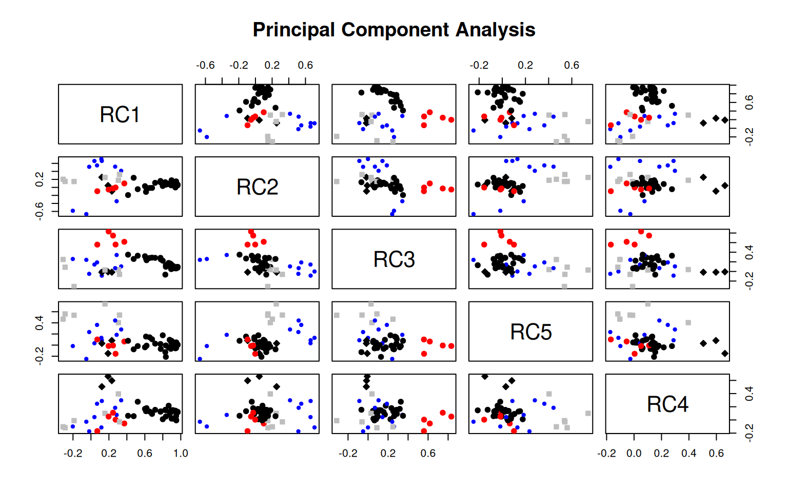
Factor analysis:
Perform a factor analysis with psych::fa. Determine how many dimensions are necessary, and justify model with goodness of fit parameters. - examine both orthogonal and non-orthogonal rotations - Create a plot showing the factor structure - examine models of different sizes to identify a good solution given the data set. - For the non-orthogonal rotation, examine correlations between factors.
Baseline solution:
efa5 <- psych::fa(r = votes, nfactors = 5)
efa5 <- psych::fa(r = votes, nfactors = 5, fm = "ols")
efa5
Factor Analysis using method = ols
Call: psych::fa(r = votes, nfactors = 5, fm = "ols")
Standardized loadings (pattern matrix) based upon correlation matrix
1 2 3 4 5 h2 u2 com
Q1 0.14 -0.03 -0.14 0.41 -0.09 0.22 0.781 1.6
Q2 0.61 0.24 0.08 0.00 -0.04 0.55 0.455 1.3
Q3 0.52 0.19 0.17 0.07 -0.24 0.49 0.506 2.0
Q4 -0.01 -0.13 0.15 0.56 0.26 0.53 0.471 1.7
Q5 -0.20 0.27 -0.07 -0.26 -0.33 0.37 0.634 3.6
Q6 0.21 0.55 0.09 0.01 0.05 0.45 0.547 1.4
Q7 0.99 -0.03 0.07 -0.11 0.00 0.92 0.082 1.0
Q8 0.68 0.19 -0.08 0.16 0.03 0.70 0.300 1.3
Q9 0.12 0.04 0.07 -0.04 0.78 0.65 0.348 1.1
[ reached 'max' / getOption("max.print") -- omitted 45 rows ]
[,1] [,2] [,3] [,4] [,5]
SS loadings 20.55 3.67 2.65 2.30 2.23
Proportion Var 0.38 0.07 0.05 0.04 0.04
Cumulative Var 0.38 0.45 0.50 0.54 0.58
Proportion Explained 0.65 0.12 0.08 0.07 0.07
Cumulative Proportion 0.65 0.77 0.86 0.93 1.00
With factor correlations of
[,1] [,2] [,3] [,4] [,5]
[1,] 1.00 0.37 0.10 0.38 0.06
[2,] 0.37 1.00 0.06 0.12 -0.14
[3,] 0.10 0.06 1.00 0.17 0.29
[4,] 0.38 0.12 0.17 1.00 0.22
[5,] 0.06 -0.14 0.29 0.22 1.00
Mean item complexity = 1.7
Test of the hypothesis that 5 factors are sufficient.
df null model = 1431 with the objective function = 88.41 with Chi Square = 8148.49
df of the model are 1171 and the objective function was 38.21
The root mean square of the residuals (RMSR) is 0.04
The df corrected root mean square of the residuals is 0.04
The harmonic n.obs is 106 with the empirical chi square 469.15 with prob < 1
The total n.obs was 112 with Likelihood Chi Square = 3394.07 with prob < 6.3e-215
Tucker Lewis Index of factoring reliability = 0.577
RMSEA index = 0.13 and the 90 % confidence intervals are 0.126 0.136
BIC = -2131.29
Fit based upon off diagonal values = 0.99
Measures of factor score adequacy
[,1] [,2] [,3] [,4] [,5]
Correlation of (regression) scores with factors 1 0.95 0.93 0.90 0.91
Multiple R square of scores with factors 1 0.91 0.87 0.81 0.83
Minimum correlation of possible factor scores 1 0.81 0.73 0.62 0.65Overall, the fit is not great (RMSEA =.13, TL=.577). These don’t change appreciably as we change the size of the model, so it indicates that the data are not well described by a factor-space model.
Factor Analysis using method =  ols
Call: psych::fa(r = votes, nfactors = 9, fm = "ols")
Standardized loadings (pattern matrix) based upon correlation matrix
       1     2     3     4     5     6     7     8     9   h2   u2 com
Q1 -0.03 -0.07  0.12  0.54 -0.06 -0.02  0.03 -0.02  0.12 0.32 0.68 1.3
Q2  0.36  0.15  0.04  0.06  0.01  0.03  0.37  0.14  0.05 0.62 0.38 2.8
Q3  0.41  0.18  0.03  0.10  0.13 -0.17  0.07  0.16  0.08 0.49 0.51 2.8
Q4 -0.16 -0.02  0.73  0.10 -0.09  0.16  0.01  0.05  0.08 0.60 0.40 1.3
Q5 -0.28  0.08 -0.46  0.13  0.09 -0.17  0.13  0.21 -0.12 0.44 0.56 3.2
Q6  0.06  0.47  0.03 -0.01  0.04  0.11  0.13  0.27 -0.03 0.49 0.51 2.0
 [ reached 'max' / getOption("max.print") -- omitted 48 rows ]

                       [,1] [,2] [,3] [,4] [,5] [,6] [,7] [,8] [,9]
SS loadings           17.84 3.42 3.10 2.13 2.07 1.93 1.76 1.74 0.76
Proportion Var         0.33 0.06 0.06 0.04 0.04 0.04 0.03 0.03 0.01
Cumulative Var         0.33 0.39 0.45 0.49 0.53 0.56 0.60 0.63 0.64
Proportion Explained   0.51 0.10 0.09 0.06 0.06 0.06 0.05 0.05 0.02
Cumulative Proportion  0.51 0.61 0.70 0.76 0.82 0.88 0.93 0.98 1.00

 With factor correlations of
      [,1]  [,2]  [,3]  [,4]  [,5]  [,6]  [,7]  [,8]  [,9]
 [1,] 1.00  0.35  0.33  0.45  0.00  0.10  0.41  0.40  0.07
 [2,] 0.35  1.00 -0.01  0.24  0.07 -0.03  0.29  0.27 -0.02
 [3,] 0.33 -0.01  1.00  0.13  0.25  0.37  0.09  0.12  0.11
 [4,] 0.45  0.24  0.13  1.00 -0.08  0.04  0.14  0.17  0.04
 [5,] 0.00  0.07  0.25 -0.08  1.00  0.22  0.00  0.02  0.02
 [6,] 0.10 -0.03  0.37  0.04  0.22  1.00 -0.04 -0.01  0.08
 [7,] 0.41  0.29  0.09  0.14  0.00 -0.04  1.00  0.16 -0.01
 [8,] 0.40  0.27  0.12  0.17  0.02 -0.01  0.16  1.00  0.02
 [ reached getOption("max.print") -- omitted 1 row ]

Mean item complexity =  2.2
Test of the hypothesis that 9 factors are sufficient.

df null model =  1431  with the objective function =  88.41 with Chi Square =  8148.49
df of  the model are 981  and the objective function was  34.58

The root mean square of the residuals (RMSR) is  0.03
The df corrected root mean square of the residuals is  0.04

The harmonic n.obs is  106 with the empirical chi square  258.06  with prob <  1
The total n.obs was  112  with Likelihood Chi Square =  2979.39  with prob <  4.4e-200

Tucker Lewis Index of factoring reliability =  0.529
RMSEA index =  0.135  and the 90 % confidence intervals are  0.13 0.141
BIC =  -1649.46
Fit based upon off diagonal values = 1
Measures of factor score adequacy
                                                  [,1] [,2] [,3] [,4] [,5] [,6]
Correlation of (regression) scores with factors      1 0.95 0.93 0.93 0.91 0.91
Multiple R square of scores with factors             1 0.90 0.86 0.86 0.82 0.83
Minimum correlation of possible factor scores        1 0.80 0.72 0.71 0.65 0.66
                                                  [,7] [,8] [,9]
Correlation of (regression) scores with factors   0.89 0.91 0.86
Multiple R square of scores with factors          0.80 0.83 0.74
Minimum correlation of possible factor scores     0.59 0.65 0.49
Here, with 9 factors, the BIC gets appreciable worse.
Factor Analysis using method =  ols
Call: psych::fa(r = votes, nfactors = 2, fm = "ols")
Standardized loadings (pattern matrix) based upon correlation matrix
        1     2    h2    u2 com
Q1   0.27  0.03 0.078 0.922 1.0
Q2   0.73 -0.04 0.521 0.479 1.0
Q3   0.67 -0.08 0.427 0.573 1.0
Q4   0.06  0.61 0.393 0.607 1.0
Q5  -0.08 -0.51 0.289 0.711 1.0
Q6   0.50 -0.05 0.238 0.762 1.0
Q7   0.93  0.02 0.869 0.131 1.0
Q8   0.83 -0.02 0.682 0.318 1.0
Q9   0.02  0.60 0.361 0.639 1.0
Q10  0.81  0.04 0.667 0.333 1.0
Q11  0.97  0.01 0.950 0.050 1.0
Q12  0.43 -0.21 0.184 0.816 1.5
Q13  0.38 -0.24 0.161 0.839 1.7
Q14  0.32  0.47 0.386 0.614 1.8
Q15  0.97  0.00 0.936 0.064 1.0
 [ reached 'max' / getOption("max.print") -- omitted 39 rows ]

                       [,1] [,2]
SS loadings           22.42 4.50
Proportion Var         0.42 0.08
Cumulative Var         0.42 0.50
Proportion Explained   0.83 0.17
Cumulative Proportion  0.83 1.00

 With factor correlations of
     [,1] [,2]
[1,] 1.00 0.23
[2,] 0.23 1.00

Mean item complexity =  1.2
Test of the hypothesis that 2 factors are sufficient.

df null model =  1431  with the objective function =  88.41 with Chi Square =  8148.49
df of  the model are 1324  and the objective function was  44.05

The root mean square of the residuals (RMSR) is  0.06
The df corrected root mean square of the residuals is  0.07

The harmonic n.obs is  106 with the empirical chi square  1193.18  with prob <  1
The total n.obs was  112  with Likelihood Chi Square =  4001.64  with prob <  2.7e-266

Tucker Lewis Index of factoring reliability =  0.561
RMSEA index =  0.134  and the 90 % confidence intervals are  0.13 0.14
BIC =  -2245.65
Fit based upon off diagonal values = 0.98
Measures of factor score adequacy
                                                  [,1] [,2]
Correlation of (regression) scores with factors   1.00 0.94
Multiple R square of scores with factors          1.00 0.89
Minimum correlation of possible factor scores     0.99 0.77
Loadings:
    [,1]   [,2]
Q1   0.271
Q2   0.730
Q3   0.667
Q4          0.611
Q5         -0.514
Q6   0.497
Q7   0.926
Q8   0.829
Q9          0.597
Q10  0.808
Q11  0.973
Q12  0.427 -0.209
Q13  0.382 -0.240
Q14  0.318  0.465
Q15  0.968
Q16  0.955
Q17  0.930
Q18  0.910
Q19  0.898
Q20  0.883
Q21  0.881
Q22  0.794
Q23  0.915
Q24  0.874 -0.110
Q25  0.625 -0.107
Q26  0.150  0.255
Q27  0.828
Q28 -0.331  0.450
Q29  0.863
Q30  0.680
Q31  0.703
Q32  0.293  0.359
Q33  0.289
Q34  0.682
Q35 -0.121  0.493
Q36  0.923
Q37  0.769
 [ reached getOption("max.print") -- omitted 17 rows ]

                 [,1]  [,2]
SS loadings    22.467 4.541
Proportion Var  0.416 0.084
Cumulative Var  0.416 0.500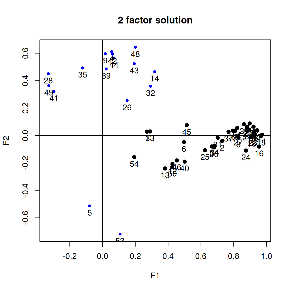
We see a similar result to earlier analyses of the Michigan House data, and it is interpretable at least for one dimension (and probably more if we were familiar with Michigan politics), but does not meet typical criteria advice about goodness of fit. This is partly because this advice comes from questionnaire and personality research, whose methods work to remove unclear questions and retain highly coherent questions that are asking essentially the same thing. In our real data set, I think the interpretability illustrates that the method can be useful even if it does not reach the statistical criteria required for personality questionnaires.