Structural Equation Modeling with lavaan
Confirmatory Factor Analysis, Latent Variable Models, Path Analysis, and Structural Equation Modeling
The set of modern methods that have their basis in PCA go by a number of different terms, including confirmatory factor analysis (CFA), structural equation modeling (SEM), latent variable modeling, latent growth models, path analysis, mediation models, and Bayesian versions of most of these. They are sometimes referred to by specific software such as AMOS, SmartPLS, mplus, and or lavaan (which is implemented in R). The methods are similar, but work in different assumptions, inference methods, and goals. The goal of this module is to provide some basic literacy in these models so that you can understand the basic principles, and be able to read and understand the literature, and build simple models for your own studies.
Additional Sources:
- http://www.phusewiki.org/docs/Conference%202013%20HE%20Papers/HE06.pdf
- https://blogs.baylor.edu/rlatentvariable/sample-page/r-syntax/
- https://methodenlehre.github.io/SGSCLM-R-course/cfa-and-sem-with-lavaan.html
- https://dominikfroehlich.com/wp-content/uploads/2018/07/Analyses-1.html
- https://stats.oarc.ucla.edu/r/seminars/rcfa/
- Making SEM diagrams: https://cran.r-project.org/web/packages/tidySEM/vignettes/sem_graph.html
- Some complete courses on SEM and CFA using lavaan: http://sachaepskamp.com/SEM2017 ## Paper comparing different packages (within and outside of R):
- https://psychology.concordia.ca/fac/kline/sem/istql/narayanan.pdf
Packages:
- lavaan
- semPlot These install a lot of additional packages for analysis and visualization.
Exploratory factor analysis (EFA) can be used to discover common underlying factors. But sometimes you might have hypotheses about the factor structure, and want to either test or confirm this in your data. The particular factor structure that come out of EFA might be the best bottom-up description, but one associated with a particular theory may be nearly as good, or perhaps even equally good, and it might be better than a description related to an alternate theory. For example, in PCA, we saw a data set created so that factors of visual and verbal intelligence emerged. The solution showed two factors, but one related to general intelligence and one that was a difference between visual and verbal. When we applied exploratory factor analysis, a rotation changed this to map more closely onto our theory, but what if we’d like to identify a particular structure (or set of alternative structures) and determine whether the data are well described by this structure? We can do this with a set of methods known as confirmatory factor analysis, structure equation modeling, and other advanced related methods. Furthermore, there may be two theories models of the structure of how processes influence one another. It can be useful to build models associated with each theory, and test which is a better description of the data.
If you are working within a factor-based framework, these models are
often called confirmatory factor analysis. That is, you
create multiple specific models that look like regression equations, but
the predictor variable is a latent, hidden variable (much like
mixture-modeling). Just like EFA with oblique rotations, you might
hypothesize there is some relationship between latent variables. We will
first cover CFA models implemented in lavaan.
But before we do, if we generalize the model to expand beyond factor models, we can create interesting theoretical models that are more complex. We could identify relationships between actual measured variables, identify latent variables, and relationships between latent variables, all using the same machinery of CFA. There are many varieties of these that go under many names; most commonly structure equation models (SEM), latent variable models, path analysis models, and specific applications like latent growth models. Furthermore, advances in hierarchical Bayes models provides substantial ability to infer latent structures. Many of these models (especially the SEM variety) still rely on correlation matrices for the data, and so even those that claim to unearth a causal structure are basing this on correlations, and are really not able to make causal inferences (this relies on experimental design, not statistical inference). Later in this unit, we will look at some of these other models.
Confirmatory Factor Analysis
Confirmatory factor analysis (CFA) is a way to create a specific factor-based latent structure and test it (usually against another latent structure) in order to compare hypotheses. Generally, you will specify the factors loading onto variables. These variables are independent factors. You can compare different numbers of factors, or different loadings. This is useful if you do a follow-up experiment after a first experiment where you conducted an EFA to identify general factors. The basic factor model still holds, but we now would specify membership of variables within factors. In EFA, a variable might have a low loading on a factor (close to 0), but in CFA we would specify that it is not part of that factor.
We will use the lavaan library for this, although other free and commercial projects exist. We will start by looking at the built-in confirmatory factor analysis example in lavaan: HolzingerSwinford1939:
This data set has nine measures that measure a number of abilties:
- x1: visual perception
- x2: cubes test
- x3: lozenges test
- x4: paragraph comprehension
- x5: sentence completion
- x6: word meaning
- x7: speeded addition
- x8: speeded counting of dots
- x9: speeded discrimination of letters
These have often been thought of having three main components: visual (x1.3), text (x4.6) and speed (x7:9).
PCA of the HolzingerSwineford1939 data:
We don’t need to start with a PCA, but let’s look at it to see what the bottom-up approach identifies:
library(lavaan)  ##needed for holzingerswineford data
data <- dplyr::select(HolzingerSwineford1939, x1:x9)
cc <- cor(data)
pca <- princomp(cc)
loadings(pca)
Loadings:
   Comp.1 Comp.2 Comp.3 Comp.4 Comp.5 Comp.6 Comp.7 Comp.8 Comp.9
x1         0.290  0.607         0.566  0.419                0.169
x2         0.522 -0.506  0.379                      -0.183  0.529
x3 -0.136  0.436  0.336 -0.549 -0.276 -0.410                0.356
x4  0.498 -0.145  0.101                0.106 -0.428 -0.715
x5  0.519 -0.184         0.175        -0.162 -0.313  0.609  0.399
x6  0.486                             -0.238  0.815 -0.142
x7 -0.273 -0.532        -0.318         0.413  0.169         0.576
x8 -0.322 -0.320  0.113  0.302  0.461 -0.610        -0.203  0.241
 [ reached getOption("max.print") -- omitted 1 row ]

               Comp.1 Comp.2 Comp.3 Comp.4 Comp.5 Comp.6 Comp.7 Comp.8 Comp.9
SS loadings     1.000  1.000  1.000  1.000  1.000  1.000  1.000  1.000  1.000
Proportion Var  0.111  0.111  0.111  0.111  0.111  0.111  0.111  0.111  0.111
Cumulative Var 0.111 0.222 0.333 0.444 0.556 0.667 0.778 0.889 1.000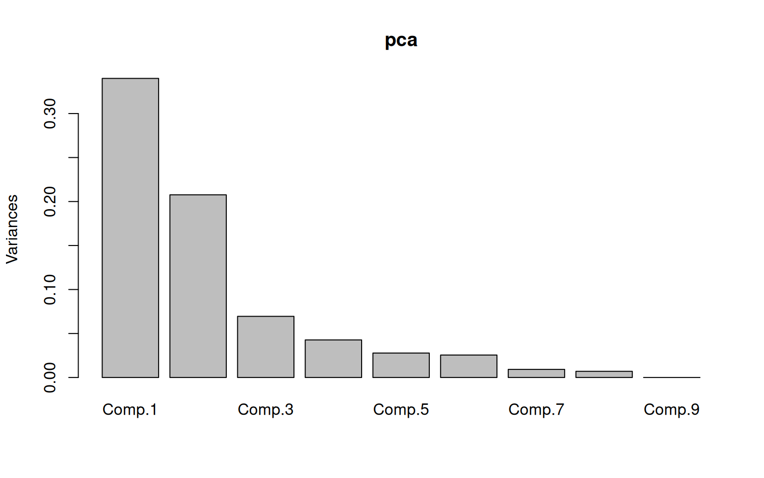 The PCA suggests that most of the variance is in the top 2 components,
with maybe the 3rd and 4th having some but lower importance.. The first
component is mostly x4, x5, and x6, which are all text-based measures.
The second component is x2, x3, and -x7, which is a comparison between
two visuo-spatial measures and addition. The third component is x1 - x2
+x9, and things get less understandable after that. The obtained
components seem to code differences between two factors, and are not
that easy to understand.
The PCA suggests that most of the variance is in the top 2 components,
with maybe the 3rd and 4th having some but lower importance.. The first
component is mostly x4, x5, and x6, which are all text-based measures.
The second component is x2, x3, and -x7, which is a comparison between
two visuo-spatial measures and addition. The third component is x1 - x2
+x9, and things get less understandable after that. The obtained
components seem to code differences between two factors, and are not
that easy to understand.
EFA of the HolzingerSwineford1939 data:
Maybe a factor analysis will be better, especially with its rotation and limited factors:
library(psych)
library(GPArotation)

f <- factanal(data, factors = 3, rotation = "oblimin", scores = "regression")
loadings(f)
Loadings:
   Factor1 Factor2 Factor3
x1  0.191   0.602
x2          0.505  -0.117
x3          0.689
x4  0.840
x5  0.888
x6  0.808
x7         -0.152   0.723
x8          0.104   0.701
x9          0.366   0.463

               Factor1 Factor2 Factor3
SS loadings      2.195   1.272   1.245
Proportion Var   0.244   0.141   0.138
Cumulative Var   0.244   0.385   0.524
With an oblique rotation, the factor structure is much cleaner. F1 is 456 (word tests), F2 is 123 (visual tests), and F3 is 789 (speeded tests).
The lavaan library confirmatory factor analysis
The name lavaan refers to latent variable analysis, which is the essence of confirmatory factor analysis. This is similar to the latent variables we used in mixture modeling (hidden group membership), as well as latent variables used in item response theory.
For simple confirmatory factor analysis, you can think of it as a set of regressions, but instead of an outcome variable, we relate observable measures to a latent variable. For lavaan, we specify a model using a special text markup that isn’t exactly R code. Enter the latent variable names on the left, the observed names on the right, separated with =~, and with each factor separated by a line break. Then, you can use the cfa function to fit it using a specified data set. The =~ operator indicates a relationship “is manifested by”, which means that the variable on the right need to actually measured. There are other relationships that you might use in more complex models.
The lavaan library has a built-in example with this same structure we discovered with EFA.
cfa> ## The famous Holzinger and Swineford (1939) example
cfa> HS.model <- ' visual  =~ x1 + x2 + x3
cfa+               textual =~ x4 + x5 + x6
cfa+               speed   =~ x7 + x8 + x9 '

cfa> fit <- cfa(HS.model, data = HolzingerSwineford1939)

cfa> summary(fit, fit.measures = TRUE)
lavaan 0.6-18 ended normally after 35 iterations

  Estimator                                         ML
  Optimization method                           NLMINB
  Number of model parameters                        21

  Number of observations                           301

Model Test User Model:

  Test statistic                                85.306
  Degrees of freedom                                24
  P-value (Chi-square)                           0.000

Model Test Baseline Model:

  Test statistic                               918.852
  Degrees of freedom                                36
  P-value                                        0.000

User Model versus Baseline Model:

  Comparative Fit Index (CFI)                    0.931
  Tucker-Lewis Index (TLI)                       0.896

Loglikelihood and Information Criteria:

  Loglikelihood user model (H0)              -3737.745
  Loglikelihood unrestricted model (H1)      -3695.092

  Akaike (AIC)                                7517.490
  Bayesian (BIC)                              7595.339
  Sample-size adjusted Bayesian (SABIC)       7528.739

Root Mean Square Error of Approximation:

  RMSEA                                          0.092
  90 Percent confidence interval - lower         0.071
  90 Percent confidence interval - upper         0.114
  P-value H_0: RMSEA <= 0.050                    0.001
  P-value H_0: RMSEA >= 0.080                    0.840

Standardized Root Mean Square Residual:

  SRMR                                           0.065

Parameter Estimates:

  Standard errors                             Standard
  Information                                 Expected
  Information saturated (h1) model          Structured

Latent Variables:
                   Estimate  Std.Err  z-value  P(>|z|)
  visual =~
    x1                1.000
    x2                0.554    0.100    5.554    0.000
    x3                0.729    0.109    6.685    0.000
  textual =~
    x4                1.000
    x5                1.113    0.065   17.014    0.000
    x6                0.926    0.055   16.703    0.000
  speed =~
    x7                1.000
    x8                1.180    0.165    7.152    0.000
    x9                1.082    0.151    7.155    0.000

Covariances:
                   Estimate  Std.Err  z-value  P(>|z|)
  visual ~~
    textual           0.408    0.074    5.552    0.000
    speed             0.262    0.056    4.660    0.000
  textual ~~
    speed             0.173    0.049    3.518    0.000

Variances:
                   Estimate  Std.Err  z-value  P(>|z|)
   .x1                0.549    0.114    4.833    0.000
   .x2                1.134    0.102   11.146    0.000
   .x3                0.844    0.091    9.317    0.000
   .x4                0.371    0.048    7.779    0.000
   .x5                0.446    0.058    7.642    0.000
   .x6                0.356    0.043    8.277    0.000
   .x7                0.799    0.081    9.823    0.000
   .x8                0.488    0.074    6.573    0.000
   .x9                0.566    0.071    8.003    0.000
    visual            0.809    0.145    5.564    0.000
    textual           0.979    0.112    8.737    0.000
    speed             0.384    0.086    4.451    0.000
We can build and fit the model ourselves. The model is specified in a
text string, and then we can fit it using the cfa
function.
HS.model <- " visual   =~ x2 + x1 + x3
              textual  =~ x4 + x5 + x6
              speed    =~ x7 + x8 + x9 "


fit <- cfa(HS.model, data = HolzingerSwineford1939)
fit
lavaan 0.6-18 ended normally after 38 iterations
Estimator ML
Optimization method NLMINB
Number of model parameters 21
Number of observations 301
Model Test User Model:
Test statistic 85.306
Degrees of freedom 24
P-value (Chi-square) 0.000lavaan 0.6-18 ended normally after 38 iterations
Estimator ML
Optimization method NLMINB
Number of model parameters 21
Number of observations 301
Model Test User Model:
Test statistic 85.306
Degrees of freedom 24
P-value (Chi-square) 0.000
Model Test Baseline Model:
Test statistic 918.852
Degrees of freedom 36
P-value 0.000
User Model versus Baseline Model:
Comparative Fit Index (CFI) 0.931
Tucker-Lewis Index (TLI) 0.896
Loglikelihood and Information Criteria:
Loglikelihood user model (H0) -3737.745
Loglikelihood unrestricted model (H1) -3695.092
Akaike (AIC) 7517.490
Bayesian (BIC) 7595.339
Sample-size adjusted Bayesian (SABIC) 7528.739
Root Mean Square Error of Approximation:
RMSEA 0.092
90 Percent confidence interval - lower 0.071
90 Percent confidence interval - upper 0.114
P-value H_0: RMSEA <= 0.050 0.001
P-value H_0: RMSEA >= 0.080 0.840
Standardized Root Mean Square Residual:
SRMR 0.065
Parameter Estimates:
Standard errors Standard
Information Expected
Information saturated (h1) model Structured
Latent Variables:
Estimate Std.Err z-value P(>|z|)
visual =~
x2 1.000
x1 1.807 0.325 5.554 0.000
x3 1.318 0.239 5.509 0.000
textual =~
x4 1.000
x5 1.113 0.065 17.014 0.000
x6 0.926 0.055 16.703 0.000
speed =~
x7 1.000
x8 1.180 0.165 7.152 0.000
x9 1.082 0.151 7.155 0.000
Covariances:
Estimate Std.Err z-value P(>|z|)
visual ~~
textual 0.226 0.052 4.329 0.000
speed 0.145 0.038 3.864 0.000
textual ~~
speed 0.173 0.049 3.518 0.000
Variances:
Estimate Std.Err z-value P(>|z|)
.x2 1.134 0.102 11.146 0.000
.x1 0.549 0.114 4.833 0.000
.x3 0.844 0.091 9.317 0.000
.x4 0.371 0.048 7.778 0.000
.x5 0.446 0.058 7.642 0.000
.x6 0.356 0.043 8.277 0.000
.x7 0.799 0.081 9.823 0.000
.x8 0.488 0.074 6.573 0.000
.x9 0.566 0.071 8.003 0.000
visual 0.248 0.077 3.214 0.001
textual 0.979 0.112 8.737 0.000
speed 0.384 0.086 4.451 0.000The above model should produce the same model that the ‘example’ did.
We can use several libraries to plot and inspect the model:
id lhs op rhs user block group free ustart exo label plabel start est
1 1 visual =~ x2 1 1 1 0 1 0 .p1. 1.000 1.000
2 2 visual =~ x1 1 1 1 1 NA 0 .p2. 1.286 1.807
3 3 visual =~ x3 1 1 1 2 NA 0 .p3. 1.424 1.318
4 4 textual =~ x4 1 1 1 0 1 0 .p4. 1.000 1.000
5 5 textual =~ x5 1 1 1 3 NA 0 .p5. 1.133 1.113
se
1 0.000
2 0.325
3 0.239
4 0.000
5 0.065
[ reached 'max' / getOption("max.print") -- omitted 19 rows ]# install.packages('semPlot',dependencies=T)
library(psych)
library(semPlot)
semPaths(fit, "model", "est", curvePivot = FALSE, edge.label.cex = 0.5)
lavaan 0.6-18 ended normally after 38 iterations

  Estimator                                         ML
  Optimization method                           NLMINB
  Number of model parameters                        21

  Number of observations                           301

Model Test User Model:

  Test statistic                                85.306
  Degrees of freedom                                24
  P-value (Chi-square)                           0.000
Model Test Baseline Model:
Test statistic 918.852
Degrees of freedom 36
P-value 0.000
User Model versus Baseline Model:
Comparative Fit Index (CFI) 0.931
Tucker-Lewis Index (TLI) 0.896
Loglikelihood and Information Criteria:
Loglikelihood user model (H0) -3737.745
Loglikelihood unrestricted model (H1) -3695.092
Akaike (AIC) 7517.490
Bayesian (BIC) 7595.339
Sample-size adjusted Bayesian (SABIC) 7528.739
Root Mean Square Error of Approximation:
RMSEA 0.092
90 Percent confidence interval - lower 0.071
90 Percent confidence interval - upper 0.114
P-value H_0: RMSEA <= 0.050 0.001
P-value H_0: RMSEA >= 0.080 0.840
Standardized Root Mean Square Residual:
SRMR 0.065
Parameter Estimates:
Standard errors Standard
Information Expected
Information saturated (h1) model Structured
Latent Variables:
Estimate Std.Err z-value P(>|z|) Std.lv Std.all
visual =~
x2 1.000 0.498 0.424
x1 1.807 0.325 5.554 0.000 0.900 0.772
x3 1.318 0.239 5.509 0.000 0.656 0.581
textual =~
x4 1.000 0.990 0.852
x5 1.113 0.065 17.014 0.000 1.102 0.855
x6 0.926 0.055 16.703 0.000 0.917 0.838
speed =~
x7 1.000 0.619 0.570
[ reached getOption("max.print") -- omitted 2 rows ]
Covariances:
Estimate Std.Err z-value P(>|z|) Std.lv Std.all
visual ~~
textual 0.226 0.052 4.329 0.000 0.459 0.459
speed 0.145 0.038 3.864 0.000 0.471 0.471
textual ~~
speed 0.173 0.049 3.518 0.000 0.283 0.283
Variances:
Estimate Std.Err z-value P(>|z|) Std.lv Std.all
.x2 1.134 0.102 11.146 0.000 1.134 0.821
.x1 0.549 0.114 4.833 0.000 0.549 0.404
.x3 0.844 0.091 9.317 0.000 0.844 0.662
.x4 0.371 0.048 7.778 0.000 0.371 0.275
.x5 0.446 0.058 7.642 0.000 0.446 0.269
.x6 0.356 0.043 8.277 0.000 0.356 0.298
.x7 0.799 0.081 9.823 0.000 0.799 0.676
.x8 0.488 0.074 6.573 0.000 0.488 0.477
.x9 0.566 0.071 8.003 0.000 0.566 0.558
visual 0.248 0.077 3.214 0.001 1.000 1.000
[ reached getOption("max.print") -- omitted 2 rows ] x2 x1 x3 x4 x5 x6 x7 x8 x9
0.179 0.596 0.338 0.725 0.731 0.702 0.324 0.523 0.442 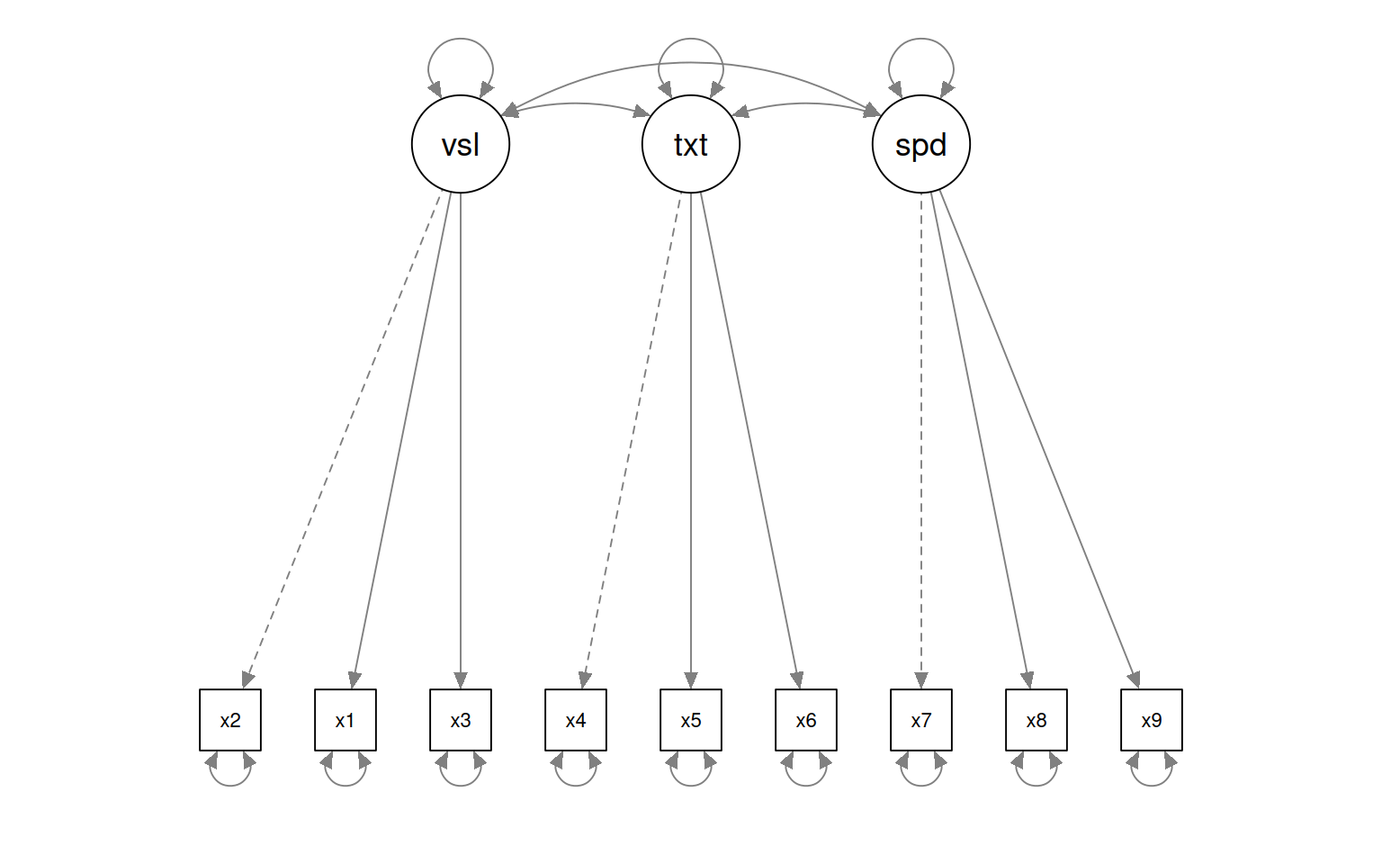
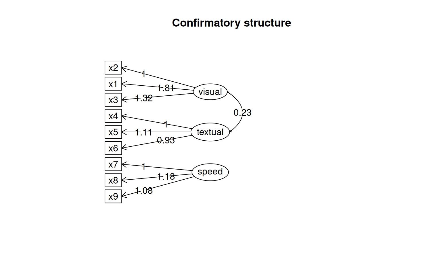
This gives some tests for whether the models are any good. First, let’s look at the diagram.
The circles indicate latent variables. The boxes indicate measured variables. two-way arrows indicate covariances; one-way arrows indicate a scaled covariance between latent and measured variables (the ~= operation), and this can be interpreted as a factor loading much like exploratory factor analysis.
Notice that for each latent variable, one loading is a dashed line, and ‘fixed’ at 1.0. This is done because there is a lack of identifiability for latent variables–you don’t really know what values they take. So by default, they are pinned to the first measure, and other loadings are expressed relative to that. So, x1 is the strongest contributor to visual performance; x5 the strongest to text, and x8 the strongest to speed. Connection that point in a circle to the same node indicate variances, and can be used to assess reliability of estimates. Finally, two-way arrows indicate covariances between latent variables. Here, we see that the relationships between the three latent variables is small but positive–with scaled covariances of .41, .26, and .17. These numbers appear in the summary() of the fitted model as well.
The summary function provides many statistics that will help interpretation. David Kenny’s page has more details on some of these that were not in standard factor analysis http://davidakenny.net/cm/fit.htm
CFI (comparative fit index) is like TLI, but will always be higher as it does not penalize complexity as much. Kenny says CFI/TLI are not meaningful unless RMSEA is below about .15. In this case RMSE is .09, which is OK but not great.
Testing alternate models
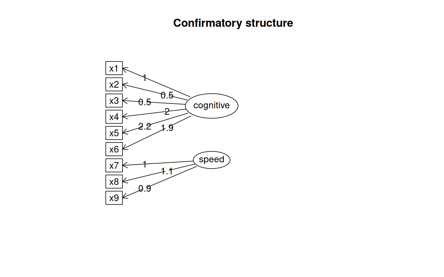
The model is reasonable, but the more powerful argument is to compare it to other models that are also reasonable. Vsl and text are correlated; maybe they really don’t belong as separate latent factors. Remember that we looked at the PCA, it didn’t look like 3 dimensions were necessary. It might be that only two are needed. Maybe really we have cognitive measures 1 through 6, and speed measures 7 through 9. We can specify that model like this:
HS.model2 <- " cognitive   =~ x1 + x2 + x3 + x4 + x5 + x6
               speed    =~ x7 + x8 + x9 "
fit2 <- cfa(HS.model2, data = HolzingerSwineford1939)
fit2
lavaan 0.6-18 ended normally after 35 iterations
Estimator ML
Optimization method NLMINB
Number of model parameters 19
Number of observations 301
Model Test User Model:
Test statistic 181.337
Degrees of freedom 26
P-value (Chi-square) 0.000lavaan 0.6-18 ended normally after 35 iterations
Estimator ML
Optimization method NLMINB
Number of model parameters 19
Number of observations 301
Model Test User Model:
Test statistic 181.337
Degrees of freedom 26
P-value (Chi-square) 0.000
Model Test Baseline Model:
Test statistic 918.852
Degrees of freedom 36
P-value 0.000
User Model versus Baseline Model:
Comparative Fit Index (CFI) 0.824
Tucker-Lewis Index (TLI) 0.756
Loglikelihood and Information Criteria:
Loglikelihood user model (H0) -3785.760
Loglikelihood unrestricted model (H1) -3695.092
Akaike (AIC) 7609.521
Bayesian (BIC) 7679.956
Sample-size adjusted Bayesian (SABIC) 7619.699
Root Mean Square Error of Approximation:
RMSEA 0.141
90 Percent confidence interval - lower 0.122
90 Percent confidence interval - upper 0.161
P-value H_0: RMSEA <= 0.050 0.000
P-value H_0: RMSEA >= 0.080 1.000
Standardized Root Mean Square Residual:
SRMR 0.113
Parameter Estimates:
Standard errors Standard
Information Expected
Information saturated (h1) model Structured
Latent Variables:
Estimate Std.Err z-value P(>|z|)
cognitive =~
x1 1.000
x2 0.509 0.156 3.254 0.001
x3 0.477 0.150 3.189 0.001
x4 1.992 0.272 7.314 0.000
x5 2.194 0.300 7.303 0.000
x6 1.852 0.254 7.294 0.000
speed =~
x7 1.000
x8 1.148 0.163 7.054 0.000
x9 0.891 0.124 7.189 0.000
Covariances:
Estimate Std.Err z-value P(>|z|)
cognitive ~~
speed 0.095 0.029 3.287 0.001
Variances:
Estimate Std.Err z-value P(>|z|)
.x1 1.112 0.093 11.922 0.000
.x2 1.318 0.108 12.193 0.000
.x3 1.219 0.100 12.196 0.000
.x4 0.373 0.047 7.853 0.000
.x5 0.474 0.059 8.059 0.000
.x6 0.351 0.043 8.221 0.000
.x7 0.732 0.083 8.821 0.000
.x8 0.428 0.082 5.201 0.000
.x9 0.658 0.071 9.300 0.000
cognitive 0.246 0.067 3.661 0.000
speed 0.451 0.095 4.733 0.000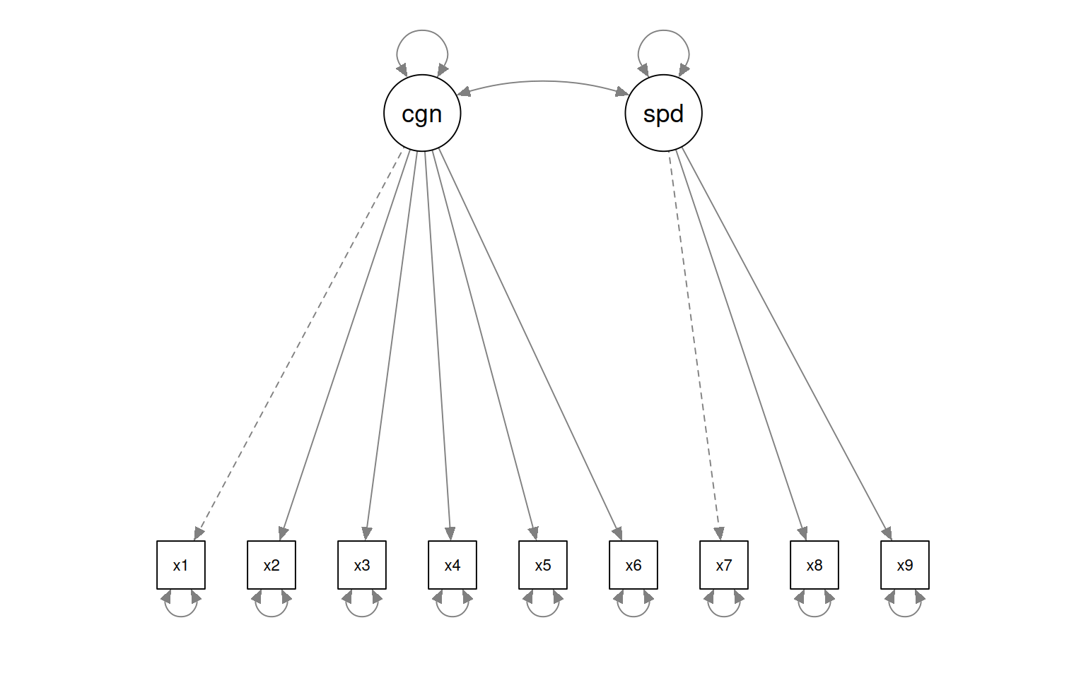
 Although we can look at specific fit measures to determine whether
either model is good, we can also compare them specifically:
Although we can look at specific fit measures to determine whether
either model is good, we can also compare them specifically:
Chi-Squared Difference Test

     Df    AIC    BIC   Chisq Chisq diff   RMSEA Df diff Pr(>Chisq)
fit  24 7517.5 7595.3  85.305
fit2 26 7609.5 7680.0 181.337     96.031 0.39522       2  < 2.2e-16 ***
---
Signif. codes:  0 '***' 0.001 '**' 0.01 '*' 0.05 '.' 0.1 ' ' 1
This shows that the two models are significantly different. The larger first model is a better fit. The chi-squared test is significant, and the AIC/BIC measures are lower for the first model, and we have just tested which factor model is better. The smaller model is fit more poorly according to RMSEA and TLI measures. Also, BIC is 7680 for the smaller model vs 7595 for the larger model, and AIC has a similar difference. Finally, anova chi-squared test is significantly different, indicating the larger model (fit) accounts for the data better than the smaller model (fit2). Altogether, this justifies the 3-factor model over the alternative 2-factor model.
We might wonder whether larger models are just going to fit better in generally. What if we give it a model we don’t think is correct–here f2 is cobbled together:
HS.model3 <- "f1  =~ x1 + x2
              f2  =~ x3 + x4
              f3  =~ x5 + x6
              f4  =~ x7 + x8 + x9 "
fit3 <- cfa(HS.model3, data = HolzingerSwineford1939)
fit3
lavaan 0.6-18 ended normally after 60 iterations
Estimator ML
Optimization method NLMINB
Number of model parameters 24
Number of observations 301
Model Test User Model:
Test statistic 144.108
Degrees of freedom 21
P-value (Chi-square) 0.000There is a warning, but it does produce a result. We can use an anova function to compare the two:
Chi-Squared Difference Test

     Df    AIC    BIC   Chisq Chisq diff RMSEA Df diff Pr(>Chisq)
fit3 21 7582.3 7671.3 144.108
fit  24 7517.5 7595.3  85.305    -58.803     0       3          1
# semPlot::semPaths(fit3,title=F,curvePilot=T)
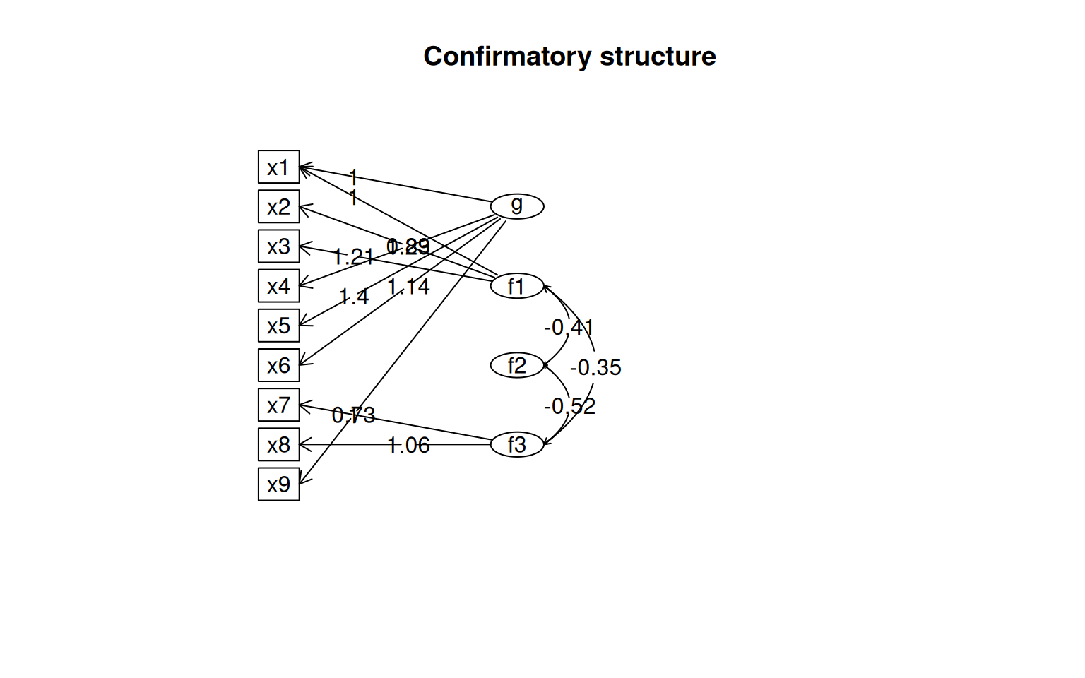
lavaan.diagram(fit3, cut = 0.2, digits = 2)
semPaths(fit3, "par", weighted = TRUE, nCharNodes = 7, shapeMan = "square", sizeMan = 8,
sizeMan2 = 5, layout = "tree2")Now, there new more complex model, which has more parameters and fewer DF,fits more poorly than the smaller model, so we would again prefer the 3-parameter model.
So, the cfa function lets us specify factor-based models directly, and compare them directly using model comparison or hypothesis testing frameworks. So it is a more intentional way of building factor-based models. Within the factor analysis framework, we can also explore overlapping factor models where measureable variables have membership in multiple factors. One–the bifactor model–is a model where all variables are related to a general factor, but also have specific factors. This is similar to the omega model we looked at before, but it is more flexible.
The Bifactor model
We previously looked at the psych::omega function, which did a EFA plus forcing a general factor g. This was proposed by Revelle as an alternative to cronbach’s alpha that could be used to identify whether a set of measures has a common structure. A confirmatory version of this is easy to do in lavaan as well, which is called the bifactor model. The bifactor model describes a model where everything is related to one general factor (g), but there are several other specific factors other things are related to. Let’s try this for the HolzingerSwineford1939 data.
## Compare to the following model, which has the same structure but it does not
## have the covariance restrictions
HS.modelG <- "G =~ x1 + x2 + x3 + x4 + x5 + x6 + x7  + x8 + x9
               visual   =~ x1 + x2 + x3
               textual =~ x4 + x5 + x6
               speed   =~ x7 + x8 + x9 "

fitG <- cfa(HS.modelG, data = HolzingerSwineford1939)
summary(fitG, fit.measures = T)
lavaan 0.6-18 ended normally after 66 iterations
Estimator ML
Optimization method NLMINB
Number of model parameters 33
Number of observations 301
Model Test User Model:
Test statistic 26.020
Degrees of freedom 12
P-value (Chi-square) 0.011
Model Test Baseline Model:
Test statistic 918.852
Degrees of freedom 36
P-value 0.000
User Model versus Baseline Model:
Comparative Fit Index (CFI) 0.984
Tucker-Lewis Index (TLI) 0.952
Loglikelihood and Information Criteria:
Loglikelihood user model (H0) -3708.102
Loglikelihood unrestricted model (H1) -3695.092
Akaike (AIC) 7482.204
Bayesian (BIC) 7604.539
Sample-size adjusted Bayesian (SABIC) 7499.882
Root Mean Square Error of Approximation:
RMSEA 0.062
90 Percent confidence interval - lower 0.029
90 Percent confidence interval - upper 0.095
P-value H_0: RMSEA <= 0.050 0.239
P-value H_0: RMSEA >= 0.080 0.206
Standardized Root Mean Square Residual:
SRMR 0.028
Parameter Estimates:
Standard errors Standard
Information Expected
Information saturated (h1) model Structured
Latent Variables:
Estimate Std.Err z-value P(>|z|)
G =~
x1 1.000
x2 0.613 NA
x3 0.768 NA
x4 0.583 NA
x5 0.552 NA
x6 0.561 NA
x7 0.442 NA
x8 0.619 NA
x9 0.699 NA
visual =~
x1 1.000
x2 0.152 NA
x3 0.127 NA
textual =~
[ reached getOption("max.print") -- omitted 7 rows ]
Covariances:
Estimate Std.Err z-value P(>|z|)
G ~~
visual -0.061 NA
textual -0.334 NA
speed -0.435 NA
visual ~~
textual 0.234 NA
speed 0.063 NA
textual ~~
speed 0.279 NA
Variances:
Estimate Std.Err z-value P(>|z|)
.x1 1.794 NA
.x2 1.025 NA
.x3 0.683 NA
.x4 0.379 NA
.x5 0.398 NA
.x6 0.368 NA
.x7 0.633 NA
.x8 0.469 NA
.x9 0.575 NA
G 1.062 NA
visual -1.377 NA
textual 1.000 NA
speed 0.727 NA
Chi-Squared Difference Test

     Df    AIC    BIC  Chisq Chisq diff   RMSEA Df diff Pr(>Chisq)
fitG 12 7482.2 7604.5 26.020
fit  24 7517.5 7595.3 85.305     59.286 0.11442      12  3.046e-08 ***
---
Signif. codes:  0 '***' 0.001 '**' 0.01 '*' 0.05 '.' 0.1 ' ' 1
Comparing the original model to this bifactor model, we have mixed results. The chi-squared test is significant suggesting the bifactor model is better, but BIC prefers the original simpler model.
HS.model4 <- "g=~ x1 + x2 + x3 + x4 + x5 + x6 + x7 + x8 + x9
               f1  =~ x1 + x2 + x3
               f2 =~ x4 + x5 + x6
               f3   =~ x7 + x8 + x9
               g ~~ 0*f1
               g ~~ 0*f2
               g ~~ 0*f3
               f1~~ 0*f1
               f2~~ 0*f2
               f3 ~~ 0*f3
"


fit4 <- cfa(HS.model4, data = HolzingerSwineford1939)
# fit4 <- cfa(HS.model4,data=HolzingerSwineford1939,estimator='WLS')
fit4
lavaan 0.6-18 ended normally after 48 iterations
Estimator ML
Optimization method NLMINB
Number of model parameters 27
Number of observations 301
Model Test User Model:
Test statistic 56.159
Degrees of freedom 18
P-value (Chi-square) 0.000lavaan 0.6-18 ended normally after 48 iterations
Estimator ML
Optimization method NLMINB
Number of model parameters 27
Number of observations 301
Model Test User Model:
Test statistic 56.159
Degrees of freedom 18
P-value (Chi-square) 0.000
Model Test Baseline Model:
Test statistic 918.852
Degrees of freedom 36
P-value 0.000
User Model versus Baseline Model:
Comparative Fit Index (CFI) 0.957
Tucker-Lewis Index (TLI) 0.914
Loglikelihood and Information Criteria:
Loglikelihood user model (H0) -3723.172
Loglikelihood unrestricted model (H1) -3695.092
Akaike (AIC) 7500.344
Bayesian (BIC) 7600.435
Sample-size adjusted Bayesian (SABIC) 7514.807
Root Mean Square Error of Approximation:
RMSEA 0.084
90 Percent confidence interval - lower 0.060
90 Percent confidence interval - upper 0.109
P-value H_0: RMSEA <= 0.050 0.013
P-value H_0: RMSEA >= 0.080 0.629
Standardized Root Mean Square Residual:
SRMR 0.051
Parameter Estimates:
Standard errors Standard
Information Expected
Information saturated (h1) model Structured
Latent Variables:
Estimate Std.Err z-value P(>|z|)
g =~
x1 1.000
x2 0.685 0.121 5.655 0.000
x3 0.921 0.151 6.118 0.000
x4 1.235 0.144 8.579 0.000
x5 1.401 0.163 8.623 0.000
x6 1.140 0.134 8.536 0.000
x7 0.841 0.125 6.746 0.000
x8 0.986 0.133 7.427 0.000
x9 0.725 0.111 6.557 0.000
f1 =~
x1 1.000
x2 0.893 0.238 3.758 0.000
x3 1.205 0.299 4.033 0.000
f2 =~
[ reached getOption("max.print") -- omitted 7 rows ]
Covariances:
Estimate Std.Err z-value P(>|z|)
g ~~
f1 0.000
f2 0.000
f3 0.000
f1 ~~
f2 -0.411 0.084 -4.897 0.000
f3 -0.349 0.081 -4.320 0.000
f2 ~~
f3 -0.523 0.084 -6.225 0.000
Variances:
Estimate Std.Err z-value P(>|z|)
f1 0.000
f2 0.000
f3 0.000
.x1 0.703 0.113 6.252 0.000
.x2 1.070 0.101 10.545 0.000
.x3 0.711 0.102 6.996 0.000
.x4 0.383 0.048 7.939 0.000
.x5 0.416 0.058 7.143 0.000
.x6 0.370 0.044 8.482 0.000
.x7 0.737 0.084 8.751 0.000
.x8 0.406 0.086 4.704 0.000
.x9 0.680 0.071 9.558 0.000
g 0.640 0.135 4.748 0.000semPaths(fit4, "par", weighted = FALSE, nCharNodes = 7, shapeMan = "rectangle", sizeMan = 8,
sizeMan2 = 5)
Here, let’s make a model removing x9 from the factor 3, but it stays in g:
HS.model4b <- "g=~ x1 + x2 + x3 + x4 + x5 + x6 + x7 + x8 + x9
f1 =~ x1 + x2 + x3
f2 =~ x4 + x5 + x6
f3 =~ x7 + x8
g ~~ 0*f1
g ~~ 0*f2
g ~~ 0*f3
f1~~ 0*f1
f2~~ 0*f2
f3 ~~ 0*f3
"
fit4b <- cfa(HS.model4b, data = HolzingerSwineford1939)
summary(fit4b, fit.measures = T)lavaan 0.6-18 ended normally after 44 iterations
Estimator ML
Optimization method NLMINB
Number of model parameters 26
Number of observations 301
Model Test User Model:
Test statistic 65.101
Degrees of freedom 19
P-value (Chi-square) 0.000
Model Test Baseline Model:
Test statistic 918.852
Degrees of freedom 36
P-value 0.000
User Model versus Baseline Model:
Comparative Fit Index (CFI) 0.948
Tucker-Lewis Index (TLI) 0.901
Loglikelihood and Information Criteria:
Loglikelihood user model (H0) -3727.643
Loglikelihood unrestricted model (H1) -3695.092
Akaike (AIC) 7507.285
Bayesian (BIC) 7603.670
Sample-size adjusted Bayesian (SABIC) 7521.213
Root Mean Square Error of Approximation:
RMSEA 0.090
90 Percent confidence interval - lower 0.066
90 Percent confidence interval - upper 0.114
P-value H_0: RMSEA <= 0.050 0.003
P-value H_0: RMSEA >= 0.080 0.769
Standardized Root Mean Square Residual:
SRMR 0.063
Parameter Estimates:
Standard errors Standard
Information Expected
Information saturated (h1) model Structured
Latent Variables:
Estimate Std.Err z-value P(>|z|)
g =~
x1 1.000
x2 0.626 0.106 5.902 0.000
x3 0.822 0.119 6.913 0.000
x4 1.173 0.122 9.591 0.000
x5 1.340 0.139 9.632 0.000
x6 1.085 0.114 9.538 0.000
x7 0.784 0.116 6.742 0.000
x8 0.932 0.127 7.363 0.000
x9 0.507 0.068 7.429 0.000
f1 =~
x1 1.000
x2 0.747 0.166 4.512 0.000
x3 0.986 0.185 5.335 0.000
f2 =~
[ reached getOption("max.print") -- omitted 6 rows ]
Covariances:
Estimate Std.Err z-value P(>|z|)
g ~~
f1 0.000
f2 0.000
f3 0.000
f1 ~~
f2 -0.434 0.075 -5.808 0.000
f3 -0.457 0.088 -5.171 0.000
f2 ~~
f3 -0.533 0.085 -6.237 0.000
Variances:
Estimate Std.Err z-value P(>|z|)
f1 0.000
f2 0.000
f3 0.000
.x1 0.618 0.105 5.867 0.000
.x2 1.091 0.100 10.855 0.000
.x3 0.773 0.091 8.450 0.000
.x4 0.387 0.048 8.063 0.000
.x5 0.419 0.058 7.224 0.000
.x6 0.370 0.043 8.546 0.000
.x7 0.723 0.096 7.563 0.000
.x8 0.375 0.107 3.500 0.000
.x9 0.827 0.062 13.266 0.000
g 0.734 0.136 5.414 0.000
Chi-Squared Difference Test
Df AIC BIC Chisq Chisq diff RMSEA Df diff Pr(>Chisq)
fit4 18 7500.3 7600.4 56.159
fit4b 19 7507.3 7603.7 65.101 8.9415 0.16243 1 0.002788 **
---
Signif. codes: 0 '***' 0.001 '**' 0.01 '*' 0.05 '.' 0.1 ' ' 1Now, the chi-squared test is significant, meaning the full bifactor model (fit4) is better, and AIC/BIC agree. Some different arguments to semPaths and lavaan.diagram can help us visualize the model.
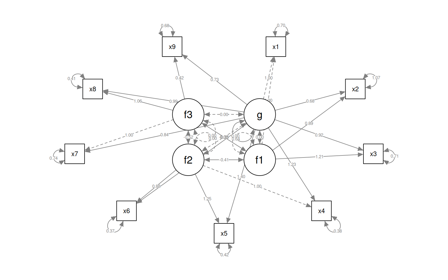
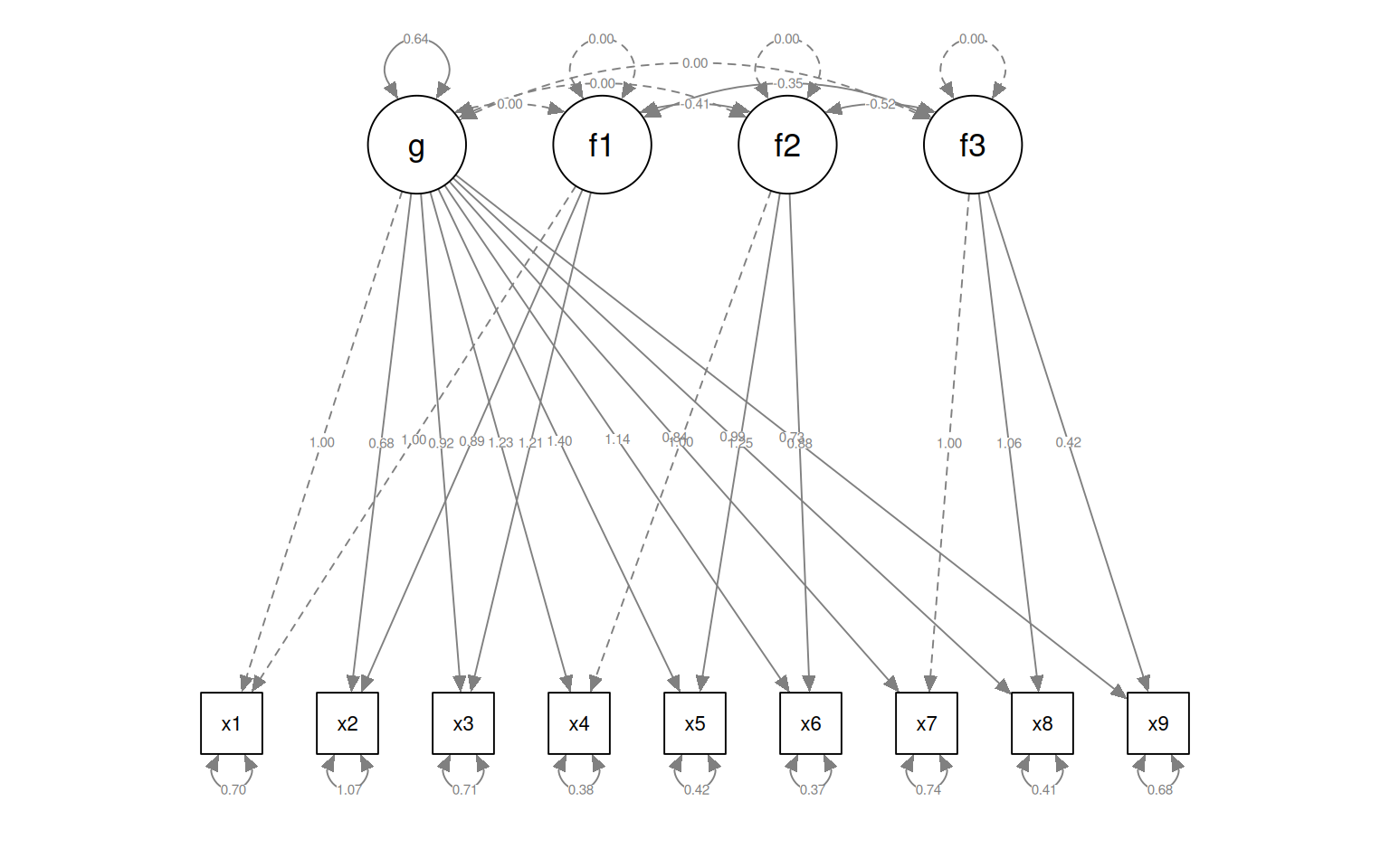
semPaths(fit4, "par", weighted = FALSE, nCharNodes = 7, shapeMan = "rectangle", sizeMan = 8,
    sizeMan2 = 5)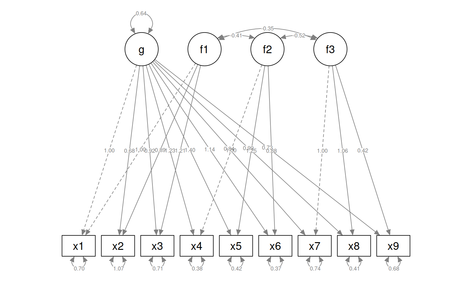
We can force the latent variables to be uncorrelated. In this case, the model does not converge, and so there is not much we can take away from it, but it might be useful in some situations. Plus, below we can see code that let’s us see the residuals of the correlation matrix, the basis for RMSE and RMSEA measures.
fit5 <- cfa(HS.model4, data = HolzingerSwineford1939, orthogonal = TRUE)
summary(fit5, fit.measures = T)
lavaan 0.6-18 ended normally after 31 iterations
Estimator ML
Optimization method NLMINB
Number of model parameters 24
Number of observations 301
Model Test User Model:
Test statistic 312.264
Degrees of freedom 21
P-value (Chi-square) 0.000
Model Test Baseline Model:
Test statistic 918.852
Degrees of freedom 36
P-value 0.000
User Model versus Baseline Model:
Comparative Fit Index (CFI) 0.670
Tucker-Lewis Index (TLI) 0.434
Loglikelihood and Information Criteria:
Loglikelihood user model (H0) -3851.224
Loglikelihood unrestricted model (H1) -3695.092
Akaike (AIC) 7750.448
Bayesian (BIC) 7839.419
Sample-size adjusted Bayesian (SABIC) 7763.305
Root Mean Square Error of Approximation:
RMSEA 0.215
90 Percent confidence interval - lower 0.194
90 Percent confidence interval - upper 0.236
P-value H_0: RMSEA <= 0.050 0.000
P-value H_0: RMSEA >= 0.080 1.000
Standardized Root Mean Square Residual:
SRMR 0.143
Parameter Estimates:
Standard errors Standard
Information Expected
Information saturated (h1) model Structured
Latent Variables:
Estimate Std.Err z-value P(>|z|)
g =~
x1 1.000
x2 0.508 NA
x3 0.493 NA
x4 1.930 NA
x5 2.123 NA
x6 1.796 NA
x7 0.385 NA
x8 0.398 NA
x9 0.606 NA
f1 =~
x1 1.000
x2 0.778 NA
x3 1.107 NA
f2 =~
[ reached getOption("max.print") -- omitted 7 rows ]
Covariances:
Estimate Std.Err z-value P(>|z|)
g ~~
f1 0.000
f2 0.000
f3 0.000
f1 ~~
f2 0.000
f3 0.000
f2 ~~
f3 0.000
Variances:
Estimate Std.Err z-value P(>|z|)
f1 0.000
f2 0.000
f3 0.000
.x1 1.098 NA
.x2 1.315 NA
.x3 1.212 NA
.x4 0.380 NA
.x5 0.486 NA
.x6 0.356 NA
.x7 1.145 NA
.x8 0.981 NA
.x9 0.919 NA
g 0.261 NA 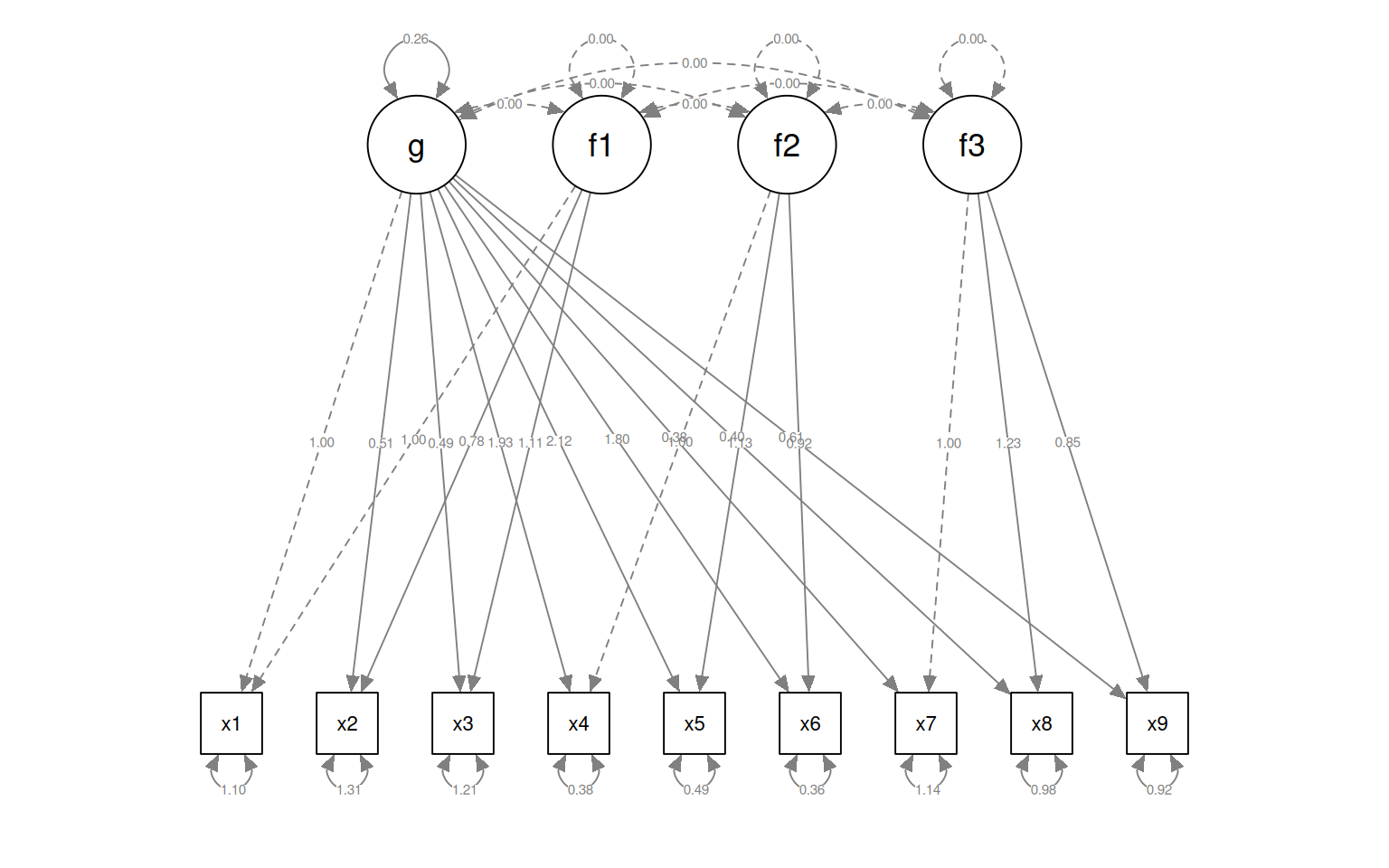
$type
[1] "cor.bollen"

$cov
       x1     x2     x3     x4     x5     x6     x7     x8     x9
x1  0.000
x2  0.201  0.000
x3  0.343  0.291  0.000
x4  0.001 -0.034 -0.030  0.000
x5 -0.075 -0.046 -0.110  0.020  0.000
x6 -0.010  0.008  0.011 -0.006  0.015  0.000
x7 -0.012 -0.115  0.032  0.021 -0.050 -0.030  0.000
x8  0.136  0.048  0.141 -0.064 -0.031 -0.019  0.450  0.000
 [ reached getOption("max.print") -- omitted 1 row ]
More on the lavaan syntax and operators
The lavaan syntax lets you describe models with 4 operators:
~Regression (structural model)=~Latent variable definition (also measurement model)~~Specifying and fixing residual correlations and covariances~1Specifying intercepts
The third operator ~~ is tricky to understand. The most
common use for this is that you are essentially adding the possibility
for measured variables to be correlated (vs uncorrelated), or forcing
them to be independent, capturing something not otherwise captured by
latent variables. You can also use coefficient notation to force
covariances to be of some value (helpful because the first covariance is
set to 1.0 in a latent model) For example, you might add
L1 ~~ 0*L2to force independence of latent variables L1 and L2.
or
L1 =~ f1 + 1*f2 + f3The ~1 operator is useful for regression-style modeling,
which is used for what are called latent growth models, used for
longitudinal, aging, and development research.
More complex models
Confirmatory factor analysis typically identifies a single set of factors and tries to model the data in that way. But the lavaan library offers more complex structural equation modeling and latent growth curve modeling, and general latent variable regressions, which is also useful in complex situations. For example, you could combine several measures to create a factor, which you then use as a regression predictor or outcome variable to establish relationships between hidden/latent variables. In developmental circles, it is common to use latent growth models to model the development or decline of specific latent cognitive or social behaviors or skills.
Path analysis and more advanced structural equation modeling
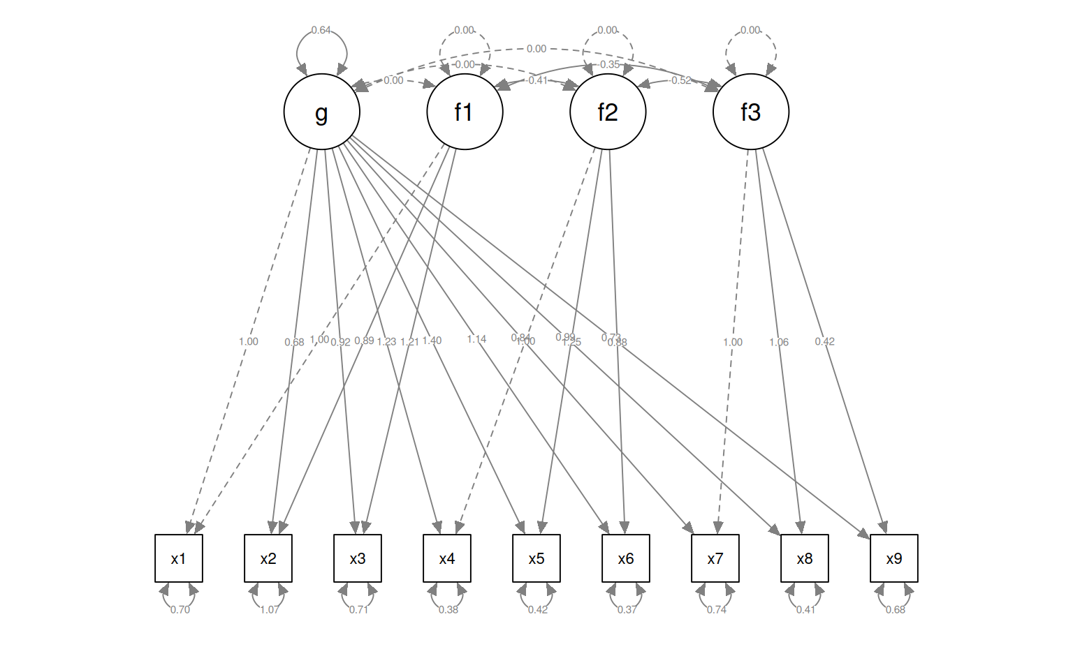
We can use the ~ operator for characterizing a covariance structure among observed variables, and compare models. The ~ is directional, so we can make complex chains and directional networks. These are really sort of sets of linear regressions. As an example, suppose we want to characterize x1 and being related to 2/3/4, 2 to 4, 3 to 4, but then x1/2/4 all being related to 5. There is a final line x5 ~~ x5 here as well, which is a covariance term. This is not necessary, but it is useful to include it in some cases.
pathAn1 <- "x1 ~ x2 + x3 + x4
           x2 ~ x4
           x3 ~ x4
           x1 + x2 +x4 ~ x5
x5 ~~ x5"

paModel <- sem(pathAn1, data = HolzingerSwineford1939)
summary(paModel, fit.measures = T)
lavaan 0.6-18 ended normally after 7 iterations
Estimator ML
Optimization method NLMINB
Number of model parameters 13
Number of observations 301
Model Test User Model:
Test statistic 34.981
Degrees of freedom 2
P-value (Chi-square) 0.000
Model Test Baseline Model:
Test statistic 392.278
Degrees of freedom 10
P-value 0.000
User Model versus Baseline Model:
Comparative Fit Index (CFI) 0.914
Tucker-Lewis Index (TLI) 0.569
Loglikelihood and Information Criteria:
Loglikelihood user model (H0) -2209.661
Loglikelihood unrestricted model (H1) -2192.171
Akaike (AIC) 4445.323
Bayesian (BIC) 4493.515
Sample-size adjusted Bayesian (SABIC) 4452.287
Root Mean Square Error of Approximation:
RMSEA 0.234
90 Percent confidence interval - lower 0.170
90 Percent confidence interval - upper 0.305
P-value H_0: RMSEA <= 0.050 0.000
P-value H_0: RMSEA >= 0.080 1.000
Standardized Root Mean Square Residual:
SRMR 0.088
Parameter Estimates:
Standard errors Standard
Information Expected
Information saturated (h1) model Structured
Regressions:
Estimate Std.Err z-value P(>|z|)
x1 ~
x2 0.129 0.048 2.685 0.007
x3 0.363 0.050 7.232 0.000
x4 0.249 0.071 3.492 0.000
x2 ~
x4 0.111 0.085 1.311 0.190
x3 ~
x4 0.154 0.055 2.788 0.005
x1 ~
x5 0.059 0.064 0.930 0.353
x2 ~
x5 0.054 0.076 0.704 0.481
x4 ~
x5 0.661 0.035 18.705 0.000
Variances:
Estimate Std.Err z-value P(>|z|)
x5 1.660 0.135 12.268 0.000
.x1 0.943 0.077 12.268 0.000
.x2 1.347 0.110 12.268 0.000
.x3 1.243 0.101 12.268 0.000
.x4 0.625 0.051 12.268 0.000semPaths(paModel, "par", weighted = FALSE, nCharNodes = 7, layout = "spring", sizeMan = 8,
sizeMan2 = 5)
This model is not very good (but that is because we are just using it as an example). However, maybe we can try an alternative. This suggests that x1 depends on 2/3/4, and 2/3/4 depend on 5.
pathAn2 <- "x1 ~ x2 + x3 + x4
            x2 + x3 + x4 ~ x5
            x5 ~~ x5"

paModel2 <- sem(pathAn2, data = HolzingerSwineford1939)
summary(paModel2, fit.measures = T)
lavaan 0.6-18 ended normally after 7 iterations
Estimator ML
Optimization method NLMINB
Number of model parameters 11
Number of observations 301
Model Test User Model:
Test statistic 43.425
Degrees of freedom 4
P-value (Chi-square) 0.000
Model Test Baseline Model:
Test statistic 392.278
Degrees of freedom 10
P-value 0.000
User Model versus Baseline Model:
Comparative Fit Index (CFI) 0.897
Tucker-Lewis Index (TLI) 0.742
Loglikelihood and Information Criteria:
Loglikelihood user model (H0) -2213.884
Loglikelihood unrestricted model (H1) -2192.171
Akaike (AIC) 4449.767
Bayesian (BIC) 4490.545
Sample-size adjusted Bayesian (SABIC) 4455.660
Root Mean Square Error of Approximation:
RMSEA 0.181
90 Percent confidence interval - lower 0.135
90 Percent confidence interval - upper 0.231
P-value H_0: RMSEA <= 0.050 0.000
P-value H_0: RMSEA >= 0.080 1.000
Standardized Root Mean Square Residual:
SRMR 0.100
Parameter Estimates:
Standard errors Standard
Information Expected
Information saturated (h1) model Structured
Regressions:
Estimate Std.Err z-value P(>|z|)
x1 ~
x2 0.132 0.048 2.764 0.006
x3 0.359 0.050 7.227 0.000
x4 0.298 0.049 6.135 0.000
x2 ~
x5 0.127 0.052 2.442 0.015
x3 ~
x5 0.068 0.050 1.343 0.179
x4 ~
x5 0.661 0.035 18.705 0.000
Variances:
Estimate Std.Err z-value P(>|z|)
x5 1.660 0.135 12.268 0.000
.x1 0.946 0.077 12.268 0.000
.x2 1.355 0.110 12.268 0.000
.x3 1.267 0.103 12.268 0.000
.x4 0.625 0.051 12.268 0.000semPaths(paModel2, "par", weighted = FALSE, nCharNodes = 7, layout = "spring", sizeMan = 8,
sizeMan2 = 5, edge.label.cex = 1)
Chi-Squared Difference Test

         Df    AIC    BIC  Chisq Chisq diff   RMSEA Df diff Pr(>Chisq)
paModel   2 4445.3 4493.5 34.981
paModel2  4 4449.8 4490.5 43.425     8.4443 0.10346       2    0.01467 *
---
Signif. codes:  0 '***' 0.001 '**' 0.01 '*' 0.05 '.' 0.1 ' ' 1
There is a significant difference between these, with model2 fitting significantly worse (but being simpler), so we’d prefer to more complex model. Note that that more complex model is not that great.
This is sort of like a simple factor analysis, and let’s you try to find a structural model that describes the relationship between observed variables, and compare it to other models. However, these models have no latent nodes–they just try to account for the covariance.
We can combine these path-style models with the latent variable models as well. This is a method generally referred to as ‘structural equation modeling’ or SEM.
Structural Equation Modeling
Structural Equation Modeling (SEM) attempts to divide the model into two parts: the measurement model and an underlying causal model relating the latent variables. The measurement model is sort of like a factor analysis: we have measured variables we want to organize into a single latent construct. The causal model is like path analysis–it models relationships between these latent variables. We will start with the CFA model earlier, but this time fit it with sem:
HS.sem <- " visual   =~ x2 + x1 + x3
             textual  =~ x4 + x5 + x6
             speed    =~ x7 + x8 + x9 "

fit_sem <- sem(HS.sem, data = HolzingerSwineford1939)
summary(fit_sem, fit.measures = T, standardized = T)
lavaan 0.6-18 ended normally after 38 iterations
Estimator ML
Optimization method NLMINB
Number of model parameters 21
Number of observations 301
Model Test User Model:
Test statistic 85.306
Degrees of freedom 24
P-value (Chi-square) 0.000
Model Test Baseline Model:
Test statistic 918.852
Degrees of freedom 36
P-value 0.000
User Model versus Baseline Model:
Comparative Fit Index (CFI) 0.931
Tucker-Lewis Index (TLI) 0.896
Loglikelihood and Information Criteria:
Loglikelihood user model (H0) -3737.745
Loglikelihood unrestricted model (H1) -3695.092
Akaike (AIC) 7517.490
Bayesian (BIC) 7595.339
Sample-size adjusted Bayesian (SABIC) 7528.739
Root Mean Square Error of Approximation:
RMSEA 0.092
90 Percent confidence interval - lower 0.071
90 Percent confidence interval - upper 0.114
P-value H_0: RMSEA <= 0.050 0.001
P-value H_0: RMSEA >= 0.080 0.840
Standardized Root Mean Square Residual:
SRMR 0.065
Parameter Estimates:
Standard errors Standard
Information Expected
Information saturated (h1) model Structured
Latent Variables:
Estimate Std.Err z-value P(>|z|) Std.lv Std.all
visual =~
x2 1.000 0.498 0.424
x1 1.807 0.325 5.554 0.000 0.900 0.772
x3 1.318 0.239 5.509 0.000 0.656 0.581
textual =~
x4 1.000 0.990 0.852
x5 1.113 0.065 17.014 0.000 1.102 0.855
x6 0.926 0.055 16.703 0.000 0.917 0.838
speed =~
x7 1.000 0.619 0.570
[ reached getOption("max.print") -- omitted 2 rows ]
Covariances:
Estimate Std.Err z-value P(>|z|) Std.lv Std.all
visual ~~
textual 0.226 0.052 4.329 0.000 0.459 0.459
speed 0.145 0.038 3.864 0.000 0.471 0.471
textual ~~
speed 0.173 0.049 3.518 0.000 0.283 0.283
Variances:
Estimate Std.Err z-value P(>|z|) Std.lv Std.all
.x2 1.134 0.102 11.146 0.000 1.134 0.821
.x1 0.549 0.114 4.833 0.000 0.549 0.404
.x3 0.844 0.091 9.317 0.000 0.844 0.662
.x4 0.371 0.048 7.778 0.000 0.371 0.275
.x5 0.446 0.058 7.642 0.000 0.446 0.269
.x6 0.356 0.043 8.277 0.000 0.356 0.298
.x7 0.799 0.081 9.823 0.000 0.799 0.676
.x8 0.488 0.074 6.573 0.000 0.488 0.477
.x9 0.566 0.071 8.003 0.000 0.566 0.558
visual 0.248 0.077 3.214 0.001 1.000 1.000
[ reached getOption("max.print") -- omitted 2 rows ]semPaths(fit_sem, what = "col", whatLabels = "std", style = "mx", rotation = 1, layout = "spring",
nCharNodes = 7, edge.label.cex = 0.9, shapeMan = "rectangle", sizeMan = 8, sizeMan2 = 5)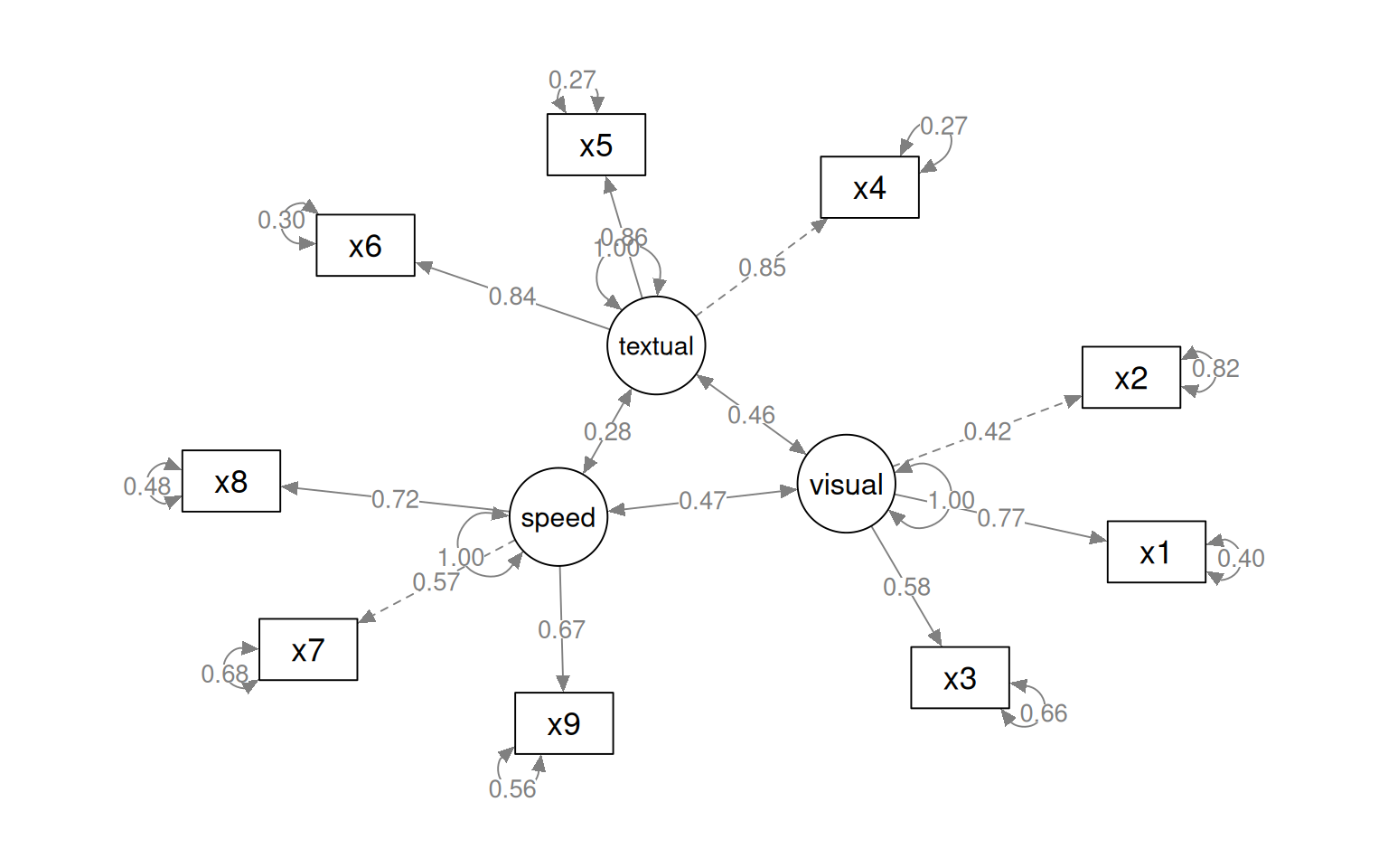
With the sem fit, we permit the different factors (now latent variables) to have correlations with other latent variables. This ends up being identical to the cfa solution, which we can see below:
semPaths(fit, what = "col", whatLabels = "std", style = "mx", rotation = 1, layout = "spring",
    nCharNodes = 7, shapeMan = "rectangle", sizeMan = 8, sizeMan2 = 5)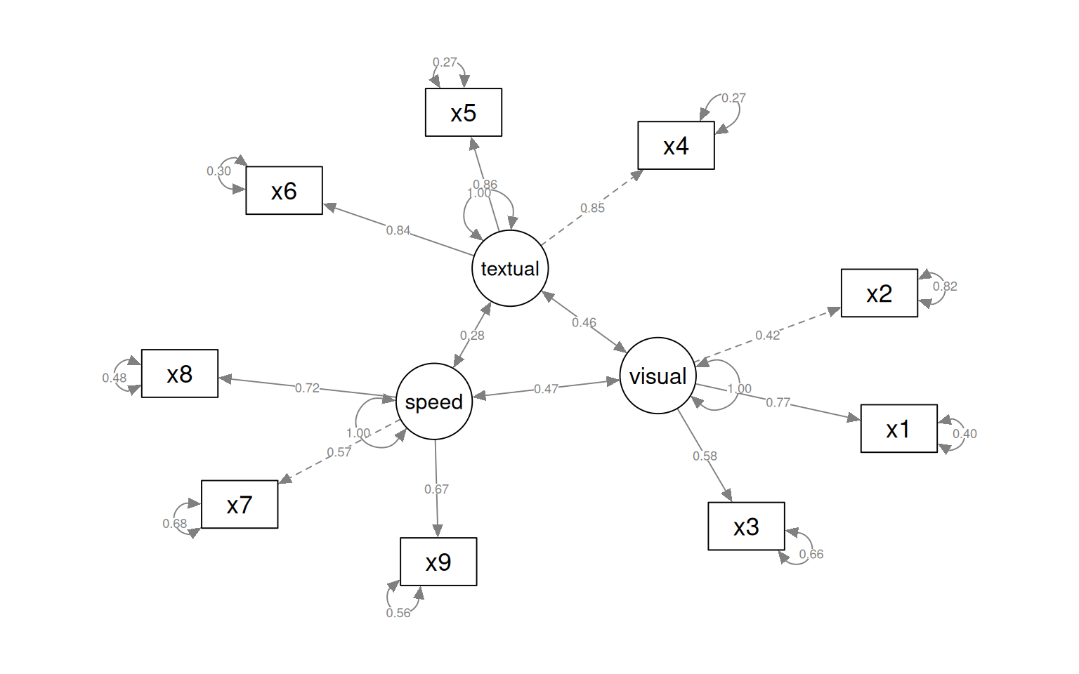
We can also specify a structural model with ~ notation. Suppose we think that textual is just visual + speed. I’ll force speed and visual to have a fixed variance and allow these to predict textual.
HS.sem2 <- " visual   =~ x2 + x1 + x3
             textual  =~ x4 + x5 + x6
             speed    =~ x7 + x8 + x9

 textual ~ visual
 visual ~  speed

"

fit_sem2 <- sem(HS.sem2, data = HolzingerSwineford1939)
summary(fit_sem2, fit.measures = T, standardized = T)
lavaan 0.6-18 ended normally after 32 iterations
Estimator ML
Optimization method NLMINB
Number of model parameters 20
Number of observations 301
Model Test User Model:
Test statistic 86.310
Degrees of freedom 25
P-value (Chi-square) 0.000
Model Test Baseline Model:
Test statistic 918.852
Degrees of freedom 36
P-value 0.000
User Model versus Baseline Model:
Comparative Fit Index (CFI) 0.931
Tucker-Lewis Index (TLI) 0.900
Loglikelihood and Information Criteria:
Loglikelihood user model (H0) -3738.247
Loglikelihood unrestricted model (H1) -3695.092
Akaike (AIC) 7516.494
Bayesian (BIC) 7590.637
Sample-size adjusted Bayesian (SABIC) 7527.208
Root Mean Square Error of Approximation:
RMSEA 0.090
90 Percent confidence interval - lower 0.070
90 Percent confidence interval - upper 0.111
P-value H_0: RMSEA <= 0.050 0.001
P-value H_0: RMSEA >= 0.080 0.806
Standardized Root Mean Square Residual:
SRMR 0.067
Parameter Estimates:
Standard errors Standard
Information Expected
Information saturated (h1) model Structured
Latent Variables:
Estimate Std.Err z-value P(>|z|) Std.lv Std.all
visual =~
x2 1.000 0.496 0.422
x1 1.801 0.321 5.613 0.000 0.894 0.767
x3 1.317 0.240 5.493 0.000 0.654 0.579
textual =~
x4 1.000 0.990 0.852
x5 1.112 0.065 17.005 0.000 1.101 0.854
x6 0.926 0.055 16.710 0.000 0.917 0.838
speed =~
x7 1.000 0.615 0.565
[ reached getOption("max.print") -- omitted 2 rows ]
Regressions:
Estimate Std.Err z-value P(>|z|) Std.lv Std.all
textual ~
visual 0.939 0.196 4.790 0.000 0.471 0.471
visual ~
speed 0.394 0.095 4.158 0.000 0.488 0.488
Variances:
Estimate Std.Err z-value P(>|z|) Std.lv Std.all
.x2 1.135 0.102 11.171 0.000 1.135 0.822
.x1 0.559 0.108 5.162 0.000 0.559 0.411
.x3 0.848 0.090 9.443 0.000 0.848 0.665
.x4 0.370 0.048 7.759 0.000 0.370 0.274
.x5 0.448 0.058 7.664 0.000 0.448 0.270
.x6 0.356 0.043 8.265 0.000 0.356 0.297
.x7 0.805 0.082 9.878 0.000 0.805 0.681
.x8 0.487 0.074 6.534 0.000 0.487 0.476
.x9 0.563 0.071 7.936 0.000 0.563 0.555
.visual 0.188 0.060 3.140 0.002 0.762 0.762
[ reached getOption("max.print") -- omitted 2 rows ]semPaths(fit_sem2, what = "col", whatLabels = "std", style = "mx", rotation = 1,
layout = "tree2", nCharNodes = 7, shapeMan = "rectangle", sizeMan = 10, sizeMan2 = 5)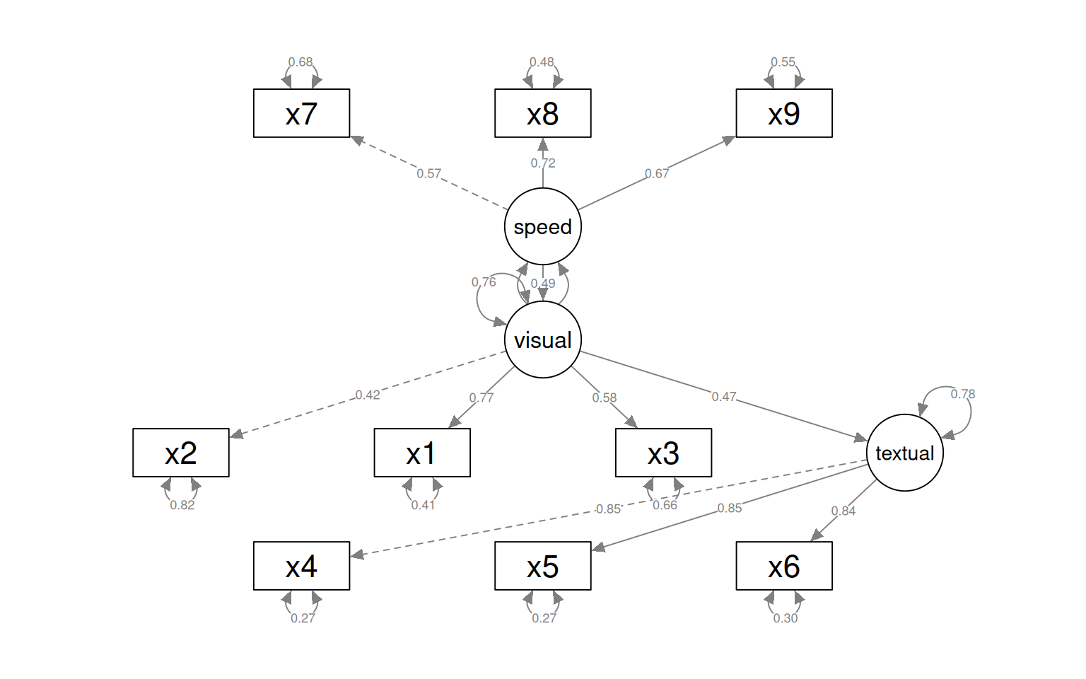
We can compare the unconstrained model to the specific causal structure we have specified. Here, we see that the unconstrained model differs significantly via the anova, so we would prefer the more complex model.
Chi-Squared Difference Test

         Df    AIC    BIC  Chisq Chisq diff     RMSEA Df diff Pr(>Chisq)
fit_sem  24 7517.5 7595.3 85.305
fit_sem2 25 7516.5 7590.6 86.310     1.0046 0.0038942       1     0.3162
Adding a structural model relating latent variables
Here, we can either include the link between speed/text, or eliminate it. this becomes like the mediation analysis (covered next time).
HS.sem3a <- " visual   =~ x2 + x1 + x3
             textual  =~ x4 + x5 + x6
             speed    =~ x7 + x8 + x9

 textual ~ a*visual + b*speed
 visual ~  c*speed

  indirect := a*b
  total := indirect + c
"

fit_sem3a <- sem(HS.sem3a, data = HolzingerSwineford1939)
summary(fit_sem3a, fit.measures = T, standardized = T)
lavaan 0.6-18 ended normally after 34 iterations
Estimator ML
Optimization method NLMINB
Number of model parameters 21
Number of observations 301
Model Test User Model:
Test statistic 85.306
Degrees of freedom 24
P-value (Chi-square) 0.000
Model Test Baseline Model:
Test statistic 918.852
Degrees of freedom 36
P-value 0.000
User Model versus Baseline Model:
Comparative Fit Index (CFI) 0.931
Tucker-Lewis Index (TLI) 0.896
Loglikelihood and Information Criteria:
Loglikelihood user model (H0) -3737.745
Loglikelihood unrestricted model (H1) -3695.092
Akaike (AIC) 7517.490
Bayesian (BIC) 7595.339
Sample-size adjusted Bayesian (SABIC) 7528.739
Root Mean Square Error of Approximation:
RMSEA 0.092
90 Percent confidence interval - lower 0.071
90 Percent confidence interval - upper 0.114
P-value H_0: RMSEA <= 0.050 0.001
P-value H_0: RMSEA >= 0.080 0.840
Standardized Root Mean Square Residual:
SRMR 0.065
Parameter Estimates:
Standard errors Standard
Information Expected
Information saturated (h1) model Structured
Latent Variables:
Estimate Std.Err z-value P(>|z|) Std.lv Std.all
visual =~
x2 1.000 0.498 0.424
x1 1.807 0.325 5.554 0.000 0.900 0.772
x3 1.318 0.239 5.509 0.000 0.656 0.581
textual =~
x4 1.000 0.990 0.852
x5 1.113 0.065 17.014 0.000 1.102 0.855
x6 0.926 0.055 16.703 0.000 0.917 0.838
speed =~
x7 1.000 0.619 0.570
[ reached getOption("max.print") -- omitted 2 rows ]
Regressions:
Estimate Std.Err z-value P(>|z|) Std.lv Std.all
textual ~
visual (a) 0.831 0.211 3.944 0.000 0.418 0.418
speed (b) 0.138 0.138 1.002 0.316 0.086 0.086
visual ~
speed (c) 0.378 0.093 4.046 0.000 0.471 0.471
Variances:
Estimate Std.Err z-value P(>|z|) Std.lv Std.all
.x2 1.134 0.102 11.146 0.000 1.134 0.821
.x1 0.549 0.114 4.833 0.000 0.549 0.404
.x3 0.844 0.091 9.317 0.000 0.844 0.662
.x4 0.371 0.048 7.779 0.000 0.371 0.275
.x5 0.446 0.058 7.642 0.000 0.446 0.269
.x6 0.356 0.043 8.277 0.000 0.356 0.298
.x7 0.799 0.081 9.823 0.000 0.799 0.676
.x8 0.488 0.074 6.573 0.000 0.488 0.477
.x9 0.566 0.071 8.003 0.000 0.566 0.558
.visual 0.193 0.061 3.150 0.002 0.779 0.779
[ reached getOption("max.print") -- omitted 2 rows ]
Defined Parameters:
Estimate Std.Err z-value P(>|z|) Std.lv Std.all
indirect 0.115 0.103 1.107 0.268 0.036 0.036
total 0.493 0.127 3.877 0.000 0.507 0.507semPaths(fit_sem3a, what = "col", whatLabels = "std", style = "mx", rotation = 1,
layout = "tree", nCharNodes = 7, shapeMan = "rectangle", sizeMan = 8, sizeMan2 = 5)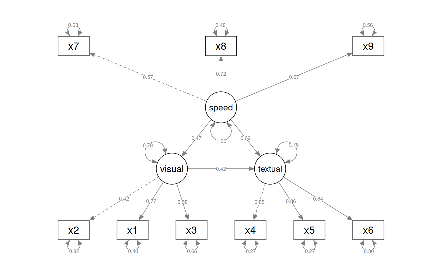
Chi-Squared Difference Test

          Df    AIC    BIC  Chisq Chisq diff     RMSEA Df diff Pr(>Chisq)
fit_sem3a 24 7517.5 7595.3 85.305
fit_sem2  25 7516.5 7590.6 86.310     1.0046 0.0038942       1     0.3162
HS.sem3 <- " visual =~ x2 + x1 + x3
textual =~ x4 + x5 + x6
speed =~ x7 + x8 + x9
textual ~ visual
visual ~ speed
"
fit_sem3 <- sem(HS.sem3, data = HolzingerSwineford1939)
summary(fit_sem3, fit.measures = T, standardized = T)lavaan 0.6-18 ended normally after 32 iterations
Estimator ML
Optimization method NLMINB
Number of model parameters 20
Number of observations 301
Model Test User Model:
Test statistic 86.310
Degrees of freedom 25
P-value (Chi-square) 0.000
Model Test Baseline Model:
Test statistic 918.852
Degrees of freedom 36
P-value 0.000
User Model versus Baseline Model:
Comparative Fit Index (CFI) 0.931
Tucker-Lewis Index (TLI) 0.900
Loglikelihood and Information Criteria:
Loglikelihood user model (H0) -3738.247
Loglikelihood unrestricted model (H1) -3695.092
Akaike (AIC) 7516.494
Bayesian (BIC) 7590.637
Sample-size adjusted Bayesian (SABIC) 7527.208
Root Mean Square Error of Approximation:
RMSEA 0.090
90 Percent confidence interval - lower 0.070
90 Percent confidence interval - upper 0.111
P-value H_0: RMSEA <= 0.050 0.001
P-value H_0: RMSEA >= 0.080 0.806
Standardized Root Mean Square Residual:
SRMR 0.067
Parameter Estimates:
Standard errors Standard
Information Expected
Information saturated (h1) model Structured
Latent Variables:
Estimate Std.Err z-value P(>|z|) Std.lv Std.all
visual =~
x2 1.000 0.496 0.422
x1 1.801 0.321 5.613 0.000 0.894 0.767
x3 1.317 0.240 5.493 0.000 0.654 0.579
textual =~
x4 1.000 0.990 0.852
x5 1.112 0.065 17.005 0.000 1.101 0.854
x6 0.926 0.055 16.710 0.000 0.917 0.838
speed =~
x7 1.000 0.615 0.565
[ reached getOption("max.print") -- omitted 2 rows ]
Regressions:
Estimate Std.Err z-value P(>|z|) Std.lv Std.all
textual ~
visual 0.939 0.196 4.790 0.000 0.471 0.471
visual ~
speed 0.394 0.095 4.158 0.000 0.488 0.488
Variances:
Estimate Std.Err z-value P(>|z|) Std.lv Std.all
.x2 1.135 0.102 11.171 0.000 1.135 0.822
.x1 0.559 0.108 5.162 0.000 0.559 0.411
.x3 0.848 0.090 9.443 0.000 0.848 0.665
.x4 0.370 0.048 7.759 0.000 0.370 0.274
.x5 0.448 0.058 7.664 0.000 0.448 0.270
.x6 0.356 0.043 8.265 0.000 0.356 0.297
.x7 0.805 0.082 9.878 0.000 0.805 0.681
.x8 0.487 0.074 6.534 0.000 0.487 0.476
.x9 0.563 0.071 7.936 0.000 0.563 0.555
.visual 0.188 0.060 3.140 0.002 0.762 0.762
[ reached getOption("max.print") -- omitted 2 rows ]semPaths(fit_sem3, what = "col", whatLabels = "std", style = "mx", rotation = 1,
layout = "tree", nCharNodes = 7, shapeMan = "rectangle", sizeMan = 8, sizeMan2 = 5)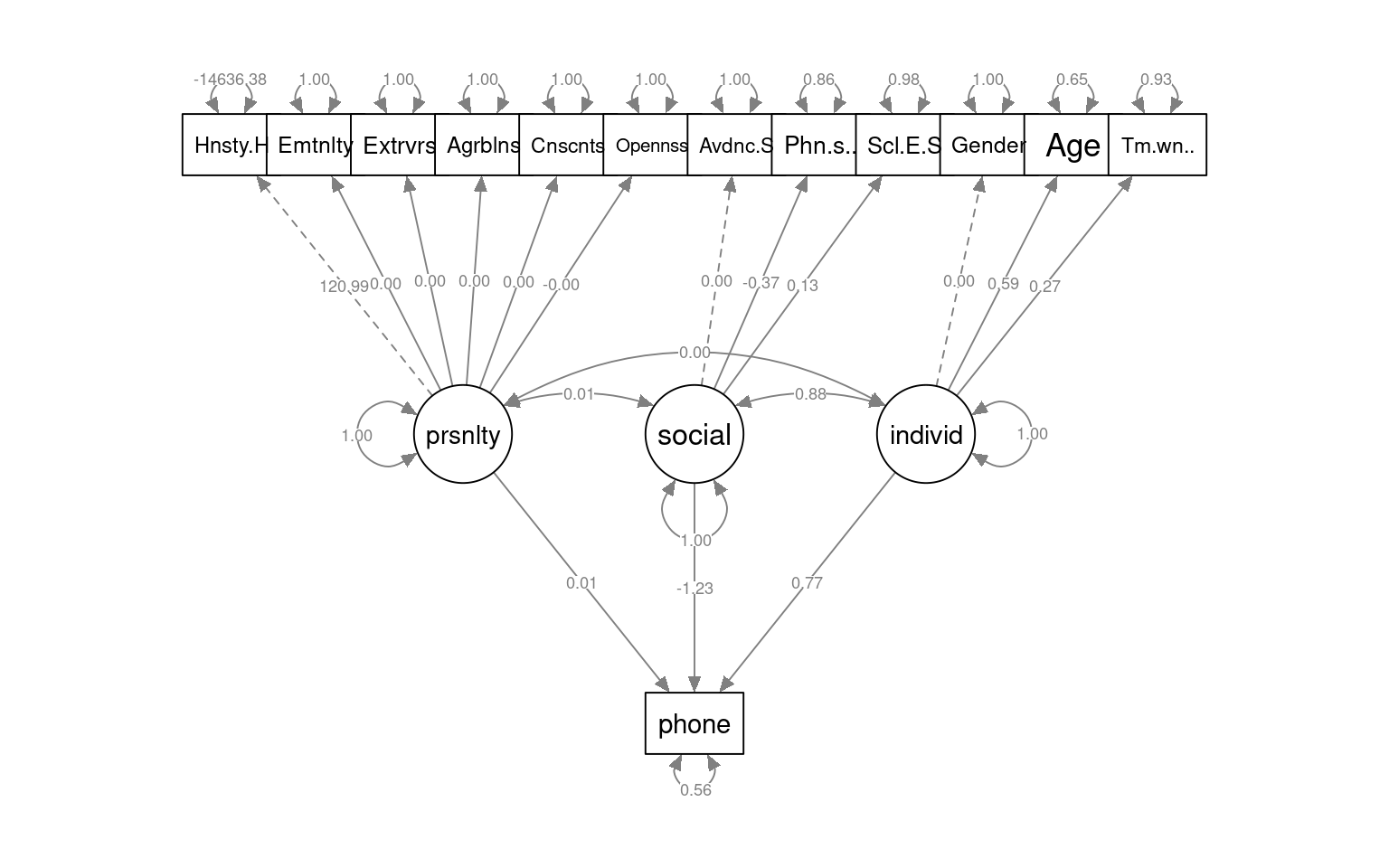
Chi-Squared Difference Test

         Df    AIC    BIC Chisq Chisq diff RMSEA Df diff Pr(>Chisq)
fit_sem3 25 7516.5 7590.6 86.31
fit_sem2 25 7516.5 7590.6 86.31          0     0       0
An Alternative structural model.
Let’s reverse the causal chain. Here, we will force speed to be predicted by visual, and visual by and textual. This is a different model, and we can compare it to the previous one.
HS.sem4 <- " visual   =~ x2 + x1 + x3
             textual  =~ x4 + x5 + x6
             speed    =~ x7 + x8 + x9

 speed ~ visual
 visual ~ textual

"

fit_sem4 <- sem(HS.sem4, data = HolzingerSwineford1939)
summary(fit_sem4, fit.measures = T, standardized = T)
lavaan 0.6-18 ended normally after 34 iterations
Estimator ML
Optimization method NLMINB
Number of model parameters 20
Number of observations 301
Model Test User Model:
Test statistic 86.310
Degrees of freedom 25
P-value (Chi-square) 0.000
Model Test Baseline Model:
Test statistic 918.852
Degrees of freedom 36
P-value 0.000
User Model versus Baseline Model:
Comparative Fit Index (CFI) 0.931
Tucker-Lewis Index (TLI) 0.900
Loglikelihood and Information Criteria:
Loglikelihood user model (H0) -3738.247
Loglikelihood unrestricted model (H1) -3695.092
Akaike (AIC) 7516.494
Bayesian (BIC) 7590.637
Sample-size adjusted Bayesian (SABIC) 7527.208
Root Mean Square Error of Approximation:
RMSEA 0.090
90 Percent confidence interval - lower 0.070
90 Percent confidence interval - upper 0.111
P-value H_0: RMSEA <= 0.050 0.001
P-value H_0: RMSEA >= 0.080 0.806
Standardized Root Mean Square Residual:
SRMR 0.067
Parameter Estimates:
Standard errors Standard
Information Expected
Information saturated (h1) model Structured
Latent Variables:
Estimate Std.Err z-value P(>|z|) Std.lv Std.all
visual =~
x2 1.000 0.496 0.422
x1 1.801 0.321 5.613 0.000 0.894 0.767
x3 1.317 0.240 5.493 0.000 0.654 0.579
textual =~
x4 1.000 0.990 0.852
x5 1.112 0.065 17.005 0.000 1.101 0.854
x6 0.926 0.055 16.710 0.000 0.917 0.838
speed =~
x7 1.000 0.615 0.565
[ reached getOption("max.print") -- omitted 2 rows ]
Regressions:
Estimate Std.Err z-value P(>|z|) Std.lv Std.all
speed ~
visual 0.604 0.143 4.212 0.000 0.488 0.488
visual ~
textual 0.236 0.050 4.739 0.000 0.471 0.471
Variances:
Estimate Std.Err z-value P(>|z|) Std.lv Std.all
.x2 1.135 0.102 11.171 0.000 1.135 0.822
.x1 0.559 0.108 5.162 0.000 0.559 0.411
.x3 0.848 0.090 9.443 0.000 0.848 0.665
.x4 0.370 0.048 7.759 0.000 0.370 0.274
.x5 0.448 0.058 7.664 0.000 0.448 0.270
.x6 0.356 0.043 8.265 0.000 0.356 0.297
.x7 0.805 0.082 9.878 0.000 0.805 0.681
.x8 0.487 0.074 6.534 0.000 0.487 0.476
.x9 0.563 0.071 7.936 0.000 0.563 0.555
.visual 0.192 0.060 3.176 0.001 0.778 0.778
[ reached getOption("max.print") -- omitted 2 rows ]semPaths(fit_sem4, what = "col", whatLabels = "std", style = "mx", rotation = 1,
layout = "tree", nCharNodes = 7, shapeMan = "rectangle", sizeMan = 8, sizeMan2 = 5)
Chi-Squared Difference Test

         Df    AIC    BIC Chisq Chisq diff RMSEA Df diff Pr(>Chisq)
fit_sem4 25 7516.5 7590.6 86.31
fit_sem3 25 7516.5 7590.6 86.31  3.739e-09     0       0
Exercise: Iphone data set
Build a SEM model that predicts the phone usage based on other predictors. Make at least two models with different sets of latent variables.
iphone <- read.csv("data_study1.csv")
iphone$phone <- as.numeric(iphone$Smartphone == "iPhone")
iphone$Gender <- iphone$Gender == "female"

iphone.base <- " personality  =~ Honesty.Humility+ Emotionality+Extraversion+Agreeableness + Conscientiousness+Openness
                  social =~ Avoidance.Similarity+Phone.as.status.object+Social.Economic.Status
                  individ =~ Gender+Age+Time.owned.current.phone

phone ~personality+social+individ
"


iphone.simple <- "social =~ Avoidance.Similarity+Phone.as.status.object+Social.Economic.Status
                  individ =~ Gender+Age+Time.owned.current.phone+Honesty.Humility+ Emotionality+Extraversion+Agreeableness + Conscientiousness+Openness

phone ~social+individ

"

iphone.simple2 <- "social =~ Avoidance.Similarity+Phone.as.status.object+Social.Economic.Status
                  individ =~ Gender+Age+Time.owned.current.phone+Honesty.Humility+ Agreeableness + Conscientiousness+Openness

phone ~social+individ+Emotionality+Extraversion
"


fit_phone1 <- sem(iphone.base, data = iphone, optim.force.converged = T)

summary(fit_phone1, fit.measures = T, standardized = T)
lavaan 0.6-18 ended normally after 2211 iterations
Estimator ML
Optimization method NLMINB
Number of model parameters 31
Number of observations 529
Model Test User Model:
Test statistic 459.401
Degrees of freedom 60
P-value (Chi-square) 0.000
Model Test Baseline Model:
Test statistic 773.724
Degrees of freedom 78
P-value 0.000
User Model versus Baseline Model:
Comparative Fit Index (CFI) 0.426
Tucker-Lewis Index (TLI) 0.254
Loglikelihood and Information Criteria:
Loglikelihood user model (H0) -9812.817
Loglikelihood unrestricted model (H1) NA
Akaike (AIC) 19687.635
Bayesian (BIC) 19820.035
Sample-size adjusted Bayesian (SABIC) 19721.633
Root Mean Square Error of Approximation:
RMSEA 0.112
90 Percent confidence interval - lower 0.103
90 Percent confidence interval - upper 0.122
P-value H_0: RMSEA <= 0.050 0.000
P-value H_0: RMSEA >= 0.080 1.000
Standardized Root Mean Square Residual:
SRMR 0.098
Parameter Estimates:
Standard errors Standard
Information Expected
Information saturated (h1) model Structured
Latent Variables:
Estimate Std.Err z-value P(>|z|) Std.lv Std.all
personality =~
Honesty.Humlty 1.000 0.513 0.820
Emotionality -0.049 NA -0.025 -0.036
Extraversion 0.091 NA 0.047 0.071
Agreeableness 0.456 NA 0.234 0.378
Conscientisnss 0.405 NA 0.208 0.343
Openness 0.205 NA 0.105 0.168
social =~
Avoidnc.Smlrty 1.000 NA NA
Phn.s.stts.bjc 2813.684 NA NA NA
[ reached getOption("max.print") -- omitted 5 rows ]
Regressions:
Estimate Std.Err z-value P(>|z|) Std.lv Std.all
phone ~
personality -0.246 NA -0.126 -0.257
social -189.787 NA NA NA
individ -1.690 NA -0.005 -0.010
Covariances:
Estimate Std.Err z-value P(>|z|) Std.lv Std.all
personality ~~
social -0.000 NA -0.463 -0.463
individ 0.000 NA 0.024 0.024
social ~~
individ -0.000 NA -0.018 -0.018
Variances:
Estimate Std.Err z-value P(>|z|) Std.lv Std.all
.Honesty.Humlty 0.128 NA 0.128 0.328
.Emotionality 0.483 NA 0.483 0.999
.Extraversion 0.429 NA 0.429 0.995
.Agreeableness 0.328 NA 0.328 0.857
.Conscientisnss 0.324 NA 0.324 0.882
.Openness 0.379 NA 0.379 0.972
.Avoidnc.Smlrty 0.694 NA 0.694 1.000
.Phn.s.stts.bjc 0.785 NA 0.785 2.229
.Scl.Ecnmc.Stts 2.343 NA 2.343 1.007
.Gender 0.223 NA 0.223 1.000
[ reached getOption("max.print") -- omitted 6 rows ]fit_phone2 <- sem(iphone.simple, data = iphone, optim.force.converged = T)
summary(fit_phone2, fit.measures = T, standardized = T)lavaan 0.6-18 ended normally after 2079 iterations
Estimator ML
Optimization method NLMINB
Number of model parameters 28
Number of observations 529
Model Test User Model:
Test statistic 446.575
Degrees of freedom 63
P-value (Chi-square) 0.000
Model Test Baseline Model:
Test statistic 773.724
Degrees of freedom 78
P-value 0.000
User Model versus Baseline Model:
Comparative Fit Index (CFI) 0.449
Tucker-Lewis Index (TLI) 0.317
Loglikelihood and Information Criteria:
Loglikelihood user model (H0) -9806.404
Loglikelihood unrestricted model (H1) NA
Akaike (AIC) 19668.809
Bayesian (BIC) 19788.397
Sample-size adjusted Bayesian (SABIC) 19699.517
Root Mean Square Error of Approximation:
RMSEA 0.107
90 Percent confidence interval - lower 0.098
90 Percent confidence interval - upper 0.117
P-value H_0: RMSEA <= 0.050 0.000
P-value H_0: RMSEA >= 0.080 1.000
Standardized Root Mean Square Residual:
SRMR 0.092
Parameter Estimates:
Standard errors Standard
Information Expected
Information saturated (h1) model Structured
Latent Variables:
Estimate Std.Err z-value P(>|z|) Std.lv Std.all
social =~
Avoidnc.Smlrty 1.000 NA NA
Phn.s.stts.bjc -56732.435 NA NA NA
Scl.Ecnmc.Stts 23718.802 NA NA NA
individ =~
Gender 1.000 0.000 0.000
Age 1065031.591 NA 5.400 0.417
Tm.wnd.crrnt.p 381068.007 NA 1.932 0.194
Honesty.Humlty 78904.406 NA 0.400 0.640
Emotionality -24510.748 NA -0.124 -0.179
[ reached getOption("max.print") -- omitted 4 rows ]
Regressions:
Estimate Std.Err z-value P(>|z|) Std.lv Std.all
phone ~
social 2254.608 NA NA NA
individ -30485.208 NA -0.155 -0.314
Covariances:
Estimate Std.Err z-value P(>|z|) Std.lv Std.all
social ~~
individ 0.000 NA 0.864 0.864
Variances:
Estimate Std.Err z-value P(>|z|) Std.lv Std.all
.Avoidnc.Smlrty 0.694 NA 0.694 1.000
.Phn.s.stts.bjc 0.543 NA 0.543 1.544
.Scl.Ecnmc.Stts 2.360 NA 2.360 1.014
.Gender 0.218 NA 0.218 1.000
.Age 138.244 NA 138.244 0.826
.Tm.wnd.crrnt.p 95.718 NA 95.718 0.962
.Honesty.Humlty 0.231 NA 0.231 0.591
.Emotionality 0.468 NA 0.468 0.968
.Extraversion 0.425 NA 0.425 0.986
.Agreeableness 0.346 NA 0.346 0.903
[ reached getOption("max.print") -- omitted 5 rows ]fit_phone3 <- sem(iphone.simple2, data = iphone, optim.force.converged = T)
summary(fit_phone3, fit.measures = T, standardized = T)lavaan 0.6-18 ended normally after 1942 iterations
Estimator ML
Optimization method NLMINB
Number of model parameters 26
Number of observations 529
Model Test User Model:
Test statistic 430.797
Degrees of freedom 62
P-value (Chi-square) 0.000
Model Test Baseline Model:
Test statistic 762.106
Degrees of freedom 77
P-value 0.000
User Model versus Baseline Model:
Comparative Fit Index (CFI) 0.462
Tucker-Lewis Index (TLI) 0.331
Loglikelihood and Information Criteria:
Loglikelihood user model (H0) -8717.848
Loglikelihood unrestricted model (H1) NA
Akaike (AIC) 17487.697
Bayesian (BIC) 17598.742
Sample-size adjusted Bayesian (SABIC) 17516.211
Root Mean Square Error of Approximation:
RMSEA 0.106
90 Percent confidence interval - lower 0.097
90 Percent confidence interval - upper 0.116
P-value H_0: RMSEA <= 0.050 0.000
P-value H_0: RMSEA >= 0.080 1.000
Standardized Root Mean Square Residual:
SRMR 0.093
Parameter Estimates:
Standard errors Standard
Information Expected
Information saturated (h1) model Structured
Latent Variables:
Estimate Std.Err z-value P(>|z|) Std.lv Std.all
social =~
Avoidnc.Smlrty 1.000 NA NA
Phn.s.stts.bjc -53567.458 NA NA NA
Scl.Ecnmc.Stts 14316.463 NA NA NA
individ =~
Gender 1.000 0.000 0.000
Age 347241.976 NA 4.822 0.373
Tm.wnd.crrnt.p 110061.133 NA 1.528 0.153
Honesty.Humlty 33285.623 NA 0.462 0.739
Agreeableness 15743.716 NA 0.219 0.353
[ reached getOption("max.print") -- omitted 2 rows ]
Regressions:
Estimate Std.Err z-value P(>|z|) Std.lv Std.all
phone ~
social 2014.046 NA NA NA
individ -10184.731 NA -0.141 -0.288
Emotionality 0.103 NA 0.103 0.145
Extraversion 0.079 NA 0.079 0.105
Covariances:
Estimate Std.Err z-value P(>|z|) Std.lv Std.all
social ~~
individ 0.000 NA 0.630 0.630
Variances:
Estimate Std.Err z-value P(>|z|) Std.lv Std.all
.Avoidnc.Smlrty 0.694 NA 0.694 1.000
.Phn.s.stts.bjc 0.651 NA 0.651 1.850
.Scl.Ecnmc.Stts 2.348 NA 2.348 1.009
.Gender 0.218 NA 0.218 1.000
.Age 144.086 NA 144.086 0.861
.Tm.wnd.crrnt.p 97.112 NA 97.112 0.977
.Honesty.Humlty 0.178 NA 0.178 0.454
.Agreeableness 0.335 NA 0.335 0.875
.Conscientisnss 0.325 NA 0.325 0.885
.Openness 0.370 NA 0.370 0.950
[ reached getOption("max.print") -- omitted 3 rows ]semPaths(fit_phone1, what = "col", whatLabels = "std", style = "mx", rotation = 1,
layout = "tree", nCharNodes = 7, shapeMan = "rectangle", sizeMan = 8, sizeMan2 = 5)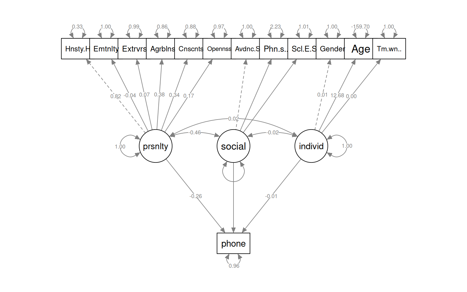
semPaths(fit_phone2, what = "col", whatLabels = "std", style = "mx", rotation = 1,
    layout = "tree", nCharNodes = 7, shapeMan = "rectangle", sizeMan = 8, sizeMan2 = 5)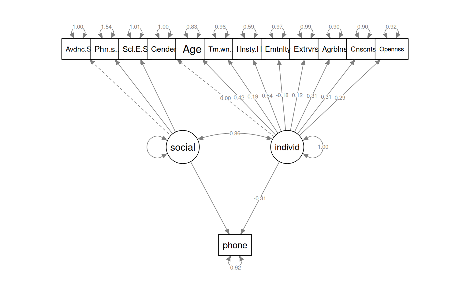
semPaths(fit_phone3, what = "col", whatLabels = "std", style = "mx", rotation = 1,
    layout = "tree", nCharNodes = 7, shapeMan = "rectangle", sizeMan = 8, sizeMan2 = 5)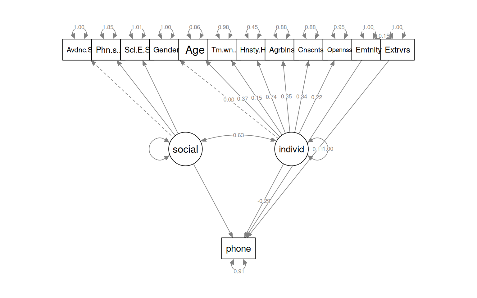
Chi-Squared Difference Test

           Df   AIC   BIC  Chisq Chisq diff RMSEA Df diff Pr(>Chisq)
fit_phone1 60 19688 19820 459.40
fit_phone2 63 19669 19788 446.58    -12.826     0       3          1
Chi-Squared Difference Test

           Df   AIC   BIC Chisq Chisq diff RMSEA Df diff Pr(>Chisq)
fit_phone1 60 19688 19820 459.4
fit_phone3 62 17488 17599 430.8 -28.605 0 2 1 df BIC
fit_phone1 31 19820.04
fit_phone2 28 19788.40
fit_phone3 26 17598.74