Correspondence Analysis and Multiple Correspondence Analysis, and Mediation Analysis
The two topics covered in this module are not related, but they are each useful in their own right.
Mediation Analysis
A common type of analysis that lavaan permits is looking at the role of mediating variables. There are many tools available for specifically looking at 3-variable problems, but lavaan lets you model arbitrarily complex mediation schemes. The analysis of these is more ad hoc though.
The notion of doing a mediation analysis is central to many areas of psychology, especially in social domains where you cannot have complete experimental control. In these cases, you will always have potentially confounding variables, and mediation analysis examines a particular kind of causal relationship. Some of the papers describing mediation are among the top 20 scientific research papers cited in any domain.
The notion is that you may observe a correlation between two variables, but also observe that these may be correlated with a third. For example, you might find that as a population ages from teenager to adult, vehicular accidents go down. But, it might not be age per se that causes this. Instead, it might be practice…as you get older, you get more experience driving, and the experience reduces accidents. Experience may be a mediating variable here. Can all the improvement in driver safety be attributed to experience? Maybe, but to find out, you need to study people who started driving at different ages. This would be a classic mediation test.
Mediation Analysis using psych::mediation
Traditionally, mediation analysis was done ‘by hand’. It involves
creating several regression models (with and without the mediator), and
comparing the residual variances, to determine how much of the
variability between the two variables is also accounted for by the
mediator. The psych library will do this for us, make a
diagram, and also carry out a number of tests and estimates of standard
error.
Below are two example data sets we can use to examine mediation. Here, using standard terminology, y is the outcome (accident rate), X is the predictor (age), and M is the mediator variable (experience). By design, in the first set, Y only depends ot X via M. In the second (Data2), M and Y depend on X independent of one another.
set.seed(1234)

X <- rnorm(100)
M <- 0.5 * X + rnorm(100)
Y <- 0.7 * M + rnorm(100)

M2 <- 0.6 * X + rnorm(100)
Y2 <- 0.6 * X + rnorm(100)


Data <- data.frame(X = X, Y = Y, M = M)
Data2 <- data.frame(X = X, Y = Y2, M = M2)

pairs(Data)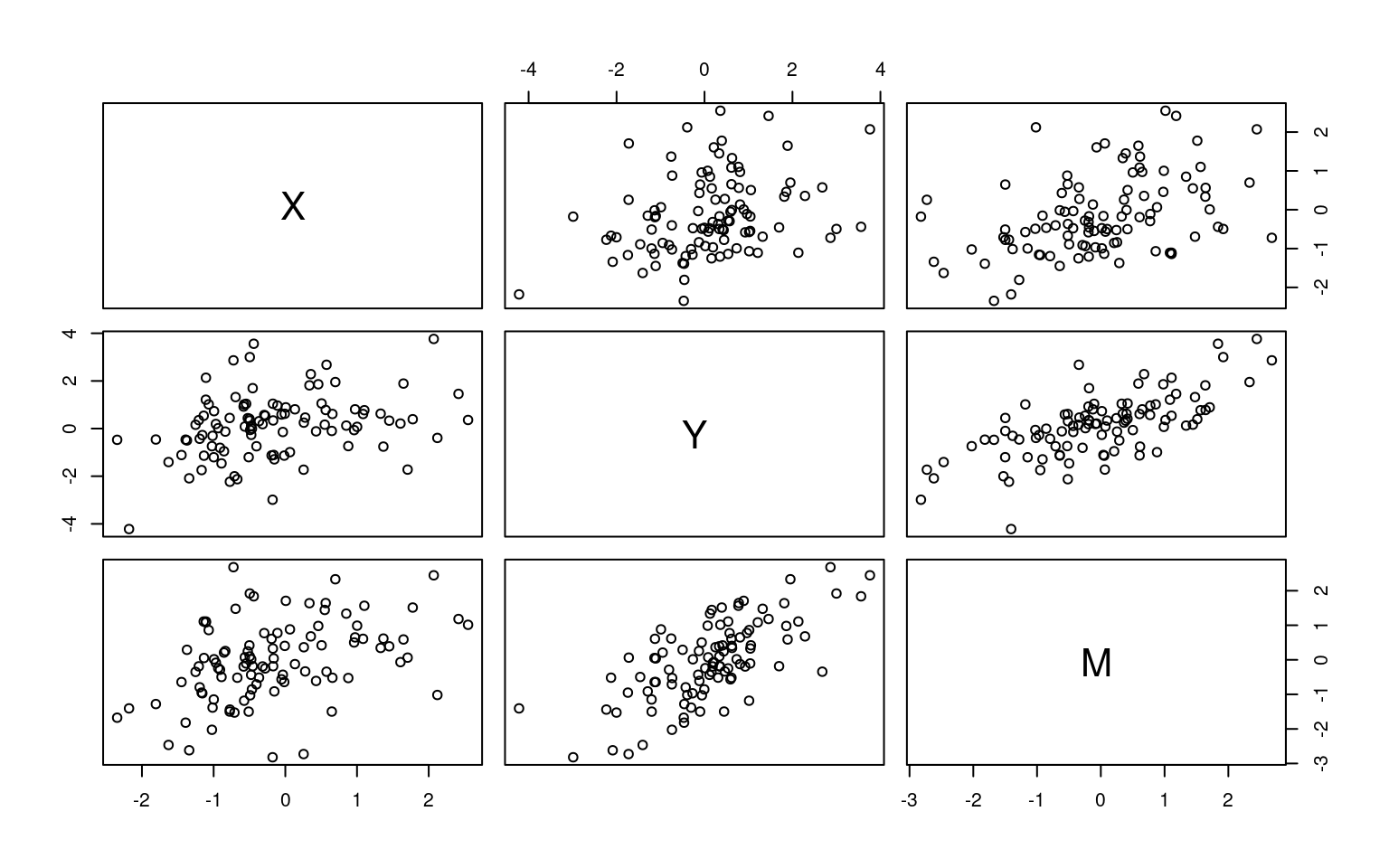
          X         Y         M
X 1.0000000 0.3122748 0.4188856
Y 0.3122748 1.0000000 0.6909791
M 0.4188856 0.6909791 1.0000000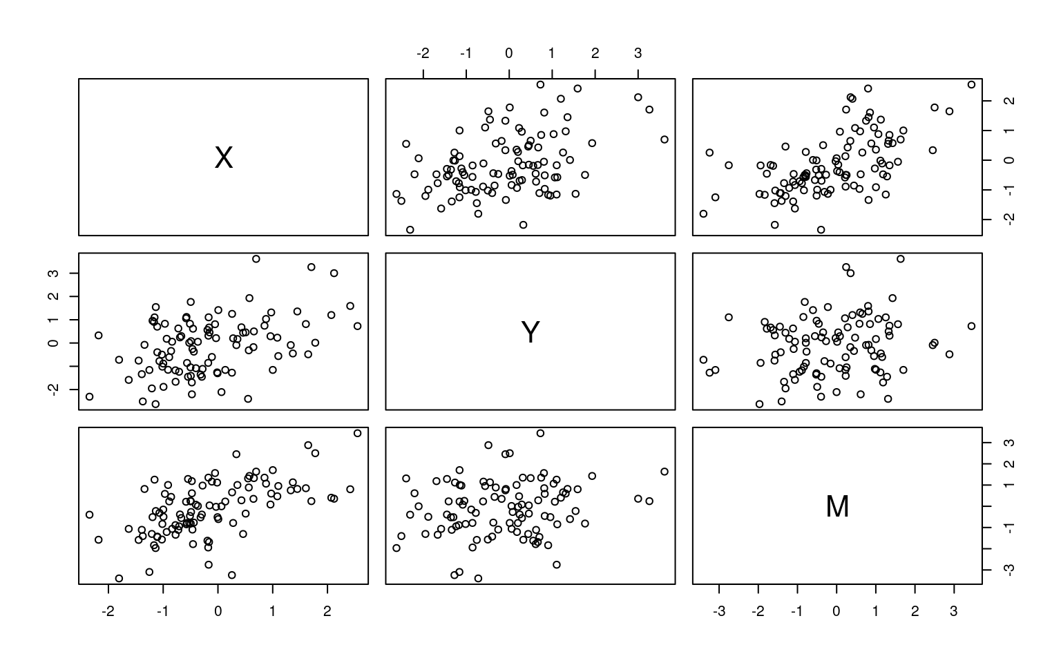
          X         Y         M
X 1.0000000 0.4255321 0.5857204
Y 0.4255321 1.0000000 0.1827901
M 0.5857204 0.1827901 1.0000000
The psych library handles standard mediation analysis using the mediate() function:

Mediation/Moderation Analysis
Call: mediate(y = Y ~ X + (M), data = Data)

The DV (Y) was  Y . The IV (X) was  X . The mediating variable(s) =  M .

Total effect(c) of  X  on  Y  =  0.41   S.E. =  0.13  t  =  3.25  df=  98   with p =  0.0016
Direct effect (c') of  X  on  Y  removing  M  =  0.04   S.E. =  0.11  t  =  0.34  df=  97   with p =  0.73
Indirect effect (ab) of  X  on  Y  through  M   =  0.37
Mean bootstrapped indirect effect =  0.37  with standard error =  0.08  Lower CI =  0.22    Upper CI =  0.54
R = 0.69 R2 = 0.48   F = 44.43 on 2 and 97 DF   p-value:  3.73e-18

 To see the longer output, specify short = FALSE in the print statement or ask for the summary
Here, the first model shows the mediated route is has substantial variance along the two legs, and the direct route c diminishes from .41 to .04 when the indirect route is allowed to have an effect, suggesting a strong mediation.
We can reverse this as well. We coefficients change but the conclusion is the same.
Mediation/Moderation Analysis
Call: mediate(y = X ~ Y + (M), data = Data)

The DV (Y) was  X . The IV (X) was  Y . The mediating variable(s) =  M .

Total effect(c) of  Y  on  X  =  0.24   S.E. =  0.07  t  =  3.25  df=  98   with p =  0.0016
Direct effect (c') of  Y  on  X  removing  M  =  0.03   S.E. =  0.1  t  =  0.34  df=  97   with p =  0.73
Indirect effect (ab) of  Y  on  X  through  M   =  0.2
Mean bootstrapped indirect effect =  0.21  with standard error =  0.07  Lower CI =  0.07    Upper CI =  0.36
R = 0.42 R2 = 0.18   F = 10.39 on 2 and 97 DF   p-value:  5.42e-06

 To see the longer output, specify short = FALSE in the print statement or ask for the summary
In Data2, the data were created so that M did not mediate Y~X.
Mediation/Moderation Analysis
Call: mediate(y = Y ~ X + (M), data = Data2)

The DV (Y) was  Y . The IV (X) was  X . The mediating variable(s) =  M .

Total effect(c) of  X  on  Y  =  0.52   S.E. =  0.11  t  =  4.66  df=  98   with p =  1e-05
Direct effect (c') of  X  on  Y  removing  M  =  0.59   S.E. =  0.14  t  =  4.29  df=  97   with p =  4.2e-05
Indirect effect (ab) of  X  on  Y  through  M   =  -0.07
Mean bootstrapped indirect effect =  -0.07  with standard error =  0.09  Lower CI =  -0.26    Upper CI =  0.09
R = 0.43 R2 = 0.19   F = 11.21 on 2 and 97 DF   p-value:  2.21e-06

 To see the longer output, specify short = FALSE in the print statement or ask for the summary
In the second model, there is no correlation along the second leg of the mediated route, and c and c’ are essentially the same, indicating M does not mediate the relationship of x to y.
So, this allows us to determine whether the mediating variable is just confounded or it is instrumental in the relationship. However, it does not really tell us causality, because the mediating relationship holds regardless of the direction.
Mediation using lavaan
So, for both Data and Data2, we have three variables that are all correlated. In truth, for Data, Y is related only to M, but M is related to X. For Data2 both M and Y are related to X directly.
We use ~ to model direct relationships between observed variables.
Here, we will fit a model with a direct relationship between X and Y,
and also another link through M. We need to specify a variable to
represent the interaction of a and b, using
:=, and a final variance total that captures
everthing.
library(lavaan)

library(semPlot)

model <- " # direct effect
Y ~ c*X
# mediator
M ~ a*X
Y ~ b*M
# indirect effect (a*b)
ab := a*b
# total effect
total := c + (a*b)
"
fitmed <- sem(model, data = Data)
summary(fitmed)
lavaan 0.6-19 ended normally after 1 iteration
Estimator ML
Optimization method NLMINB
Number of model parameters 5
Number of observations 100
Model Test User Model:
Test statistic 0.000
Degrees of freedom 0
Parameter Estimates:
Standard errors Standard
Information Expected
Information saturated (h1) model Structured
Regressions:
Estimate Std.Err z-value P(>|z|)
Y ~
X (c) 0.036 0.104 0.348 0.728
M ~
X (a) 0.474 0.103 4.613 0.000
Y ~
M (b) 0.788 0.092 8.539 0.000
Variances:
Estimate Std.Err z-value P(>|z|)
.Y 0.898 0.127 7.071 0.000
.M 1.054 0.149 7.071 0.000
Defined Parameters:
Estimate Std.Err z-value P(>|z|)
ab 0.374 0.092 4.059 0.000
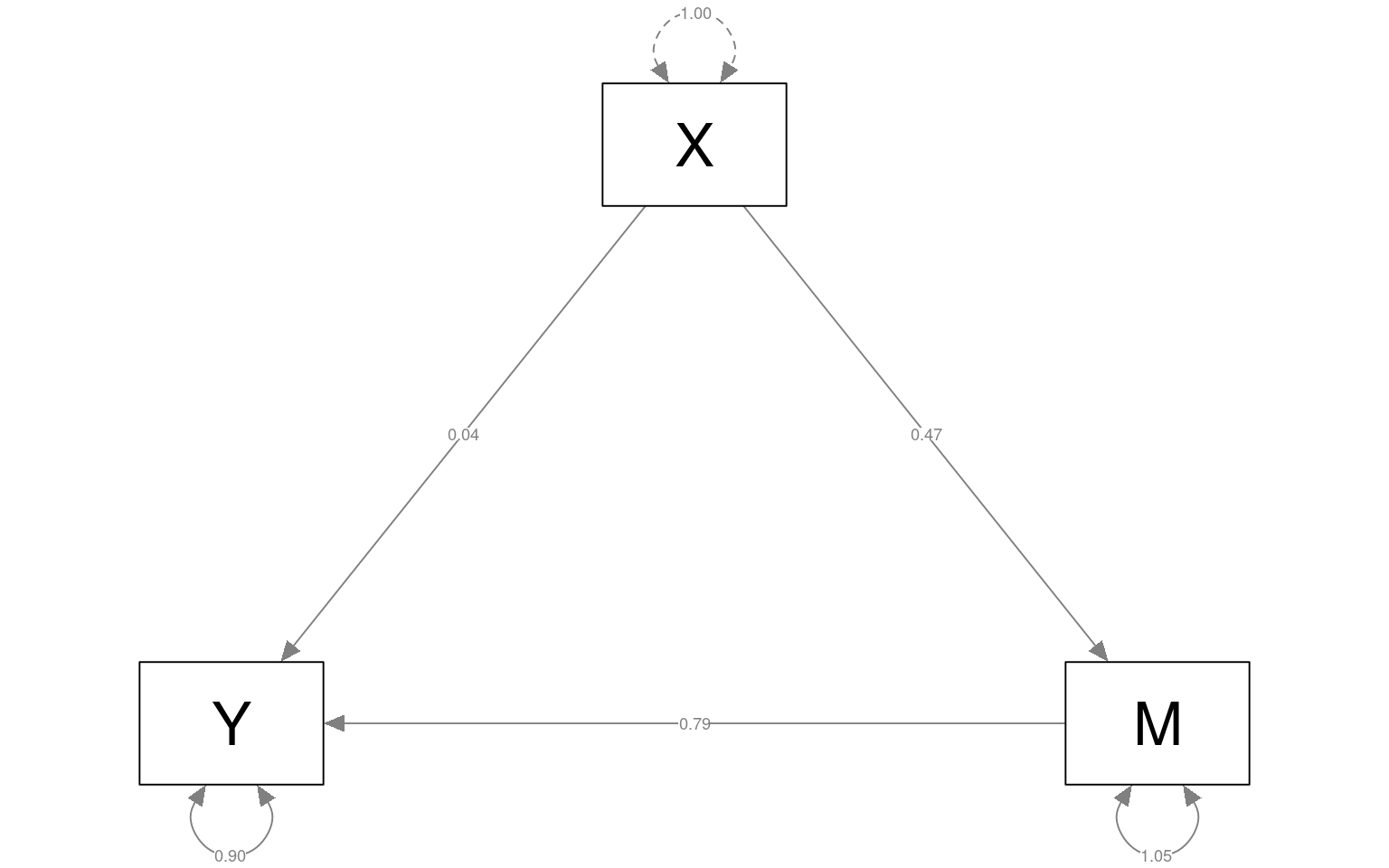
total 0.410 0.125 3.287 0.001semPaths(fitmed, curvePilot = T, "par", weighted = FALSE, nCharNodes = 7, shapeMan = "rectangle",
sizeMan = 15, sizeMan2 = 10)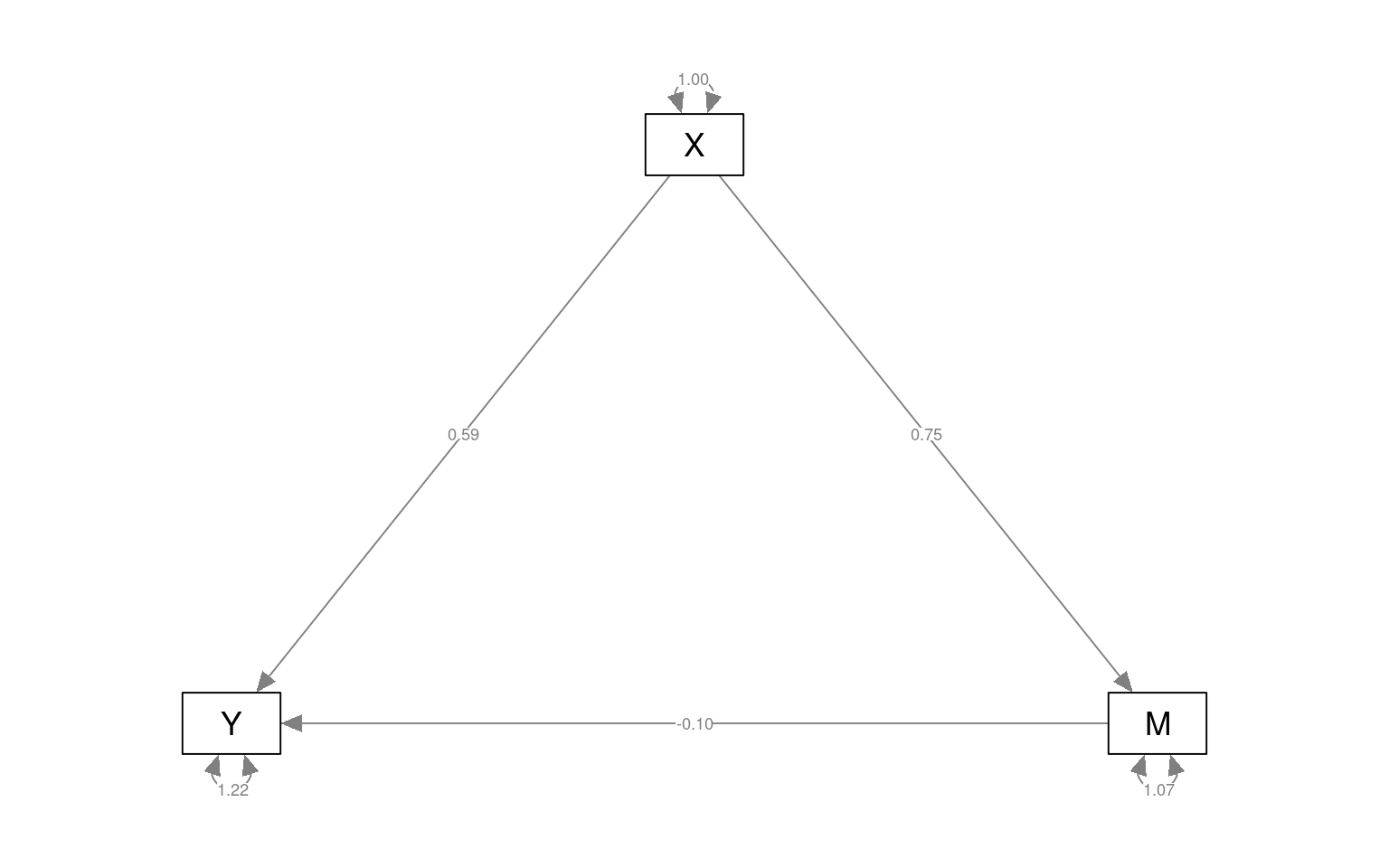
Looking at this first model (where M really mediates X-Y), we see that the edges X-M and M-Y are strong, but X->Y is weak, indicating M mediates the relationship between X and Y. These values are nearly identical (if not exactly the same) to what we obtained in the mediate function, with c=total=.41, but the lavaan model gives more details.
lavaan 0.6-19 ended normally after 1 iteration

  Estimator                                         ML
  Optimization method                           NLMINB
  Number of model parameters                         5

  Number of observations                           100

Model Test User Model:

  Test statistic                                 0.000
  Degrees of freedom                                 0

Parameter Estimates:

  Standard errors                             Standard
  Information                                 Expected
  Information saturated (h1) model          Structured

Regressions:
                   Estimate  Std.Err  z-value  P(>|z|)
  Y ~
    X          (c)    0.594    0.136    4.360    0.000
  M ~
    X          (a)    0.748    0.104    7.227    0.000
  Y ~
    M          (b)   -0.097    0.107   -0.910    0.363

Variances:
                   Estimate  Std.Err  z-value  P(>|z|)
   .Y                 1.218    0.172    7.071    0.000
   .M                 1.070    0.151    7.071    0.000

Defined Parameters:
                   Estimate  Std.Err  z-value  P(>|z|)
    ab               -0.073    0.080   -0.903    0.367
    total             0.521    0.111    4.702    0.000
# lavaan.diagram(fit2)
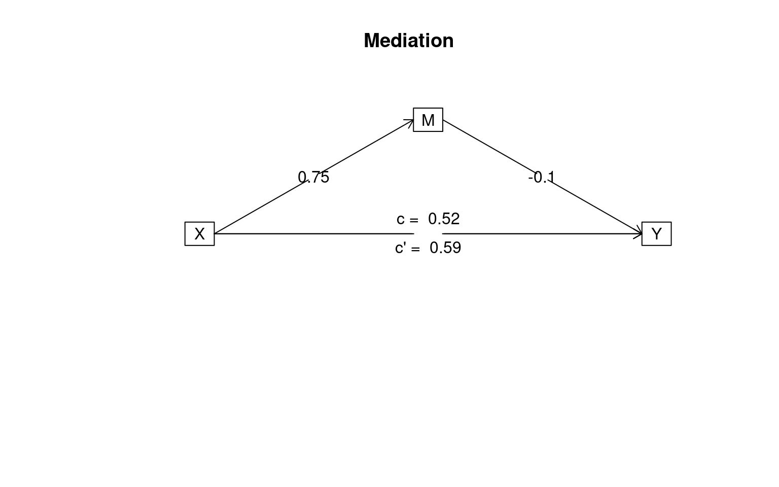
semPaths(fitmed2, curvePilot = T, "par", weighted = FALSE, nCharNodes = 7, shapeMan = "rectangle",
sizeMan = 8, sizeMan2 = 5)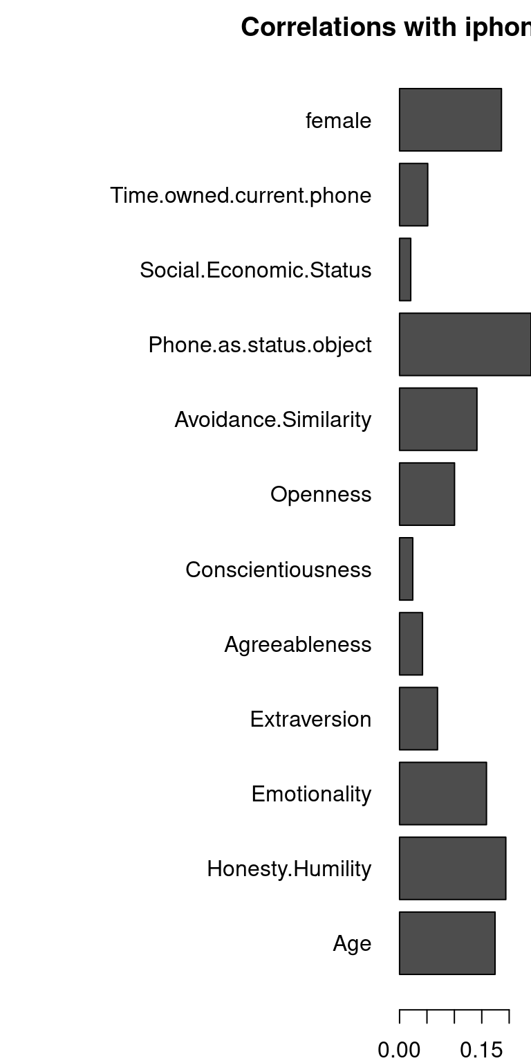 Here, Y-M is not significant, but Y-X and M-X are, indicating that M
does not mediate the relationship. Note that the model is framed to test
whether a particular value is significant–we don’t make two models and
compare theme via ANOVA.
Here, Y-M is not significant, but Y-X and M-X are, indicating that M
does not mediate the relationship. Note that the model is framed to test
whether a particular value is significant–we don’t make two models and
compare theme via ANOVA.
Example: Iphone data
dat <- read.csv("data_study1.csv")
dat$female <- dat$Gender == "female"
dat$phonenumeric <- dat$Smartphone == "iPhone"
round(cor(dat$phonenumeric, dat[, 3:14]), 2)
Age Honesty.Humility Emotionality Extraversion Agreeableness
[1,] -0.17 -0.19 0.16 0.07 -0.04
Conscientiousness Openness Avoidance.Similarity Phone.as.status.object
[1,] 0.02 -0.1 -0.14 0.24
Social.Economic.Status Time.owned.current.phone female
[1,] 0.02 -0.05 0.19par(mar = c(2, 15, 2, 0))
barplot(abs(cor(dat$phonenumeric, dat[, 3:14])), main = "Correlations with iphone ownership",
horiz = T, las = 1)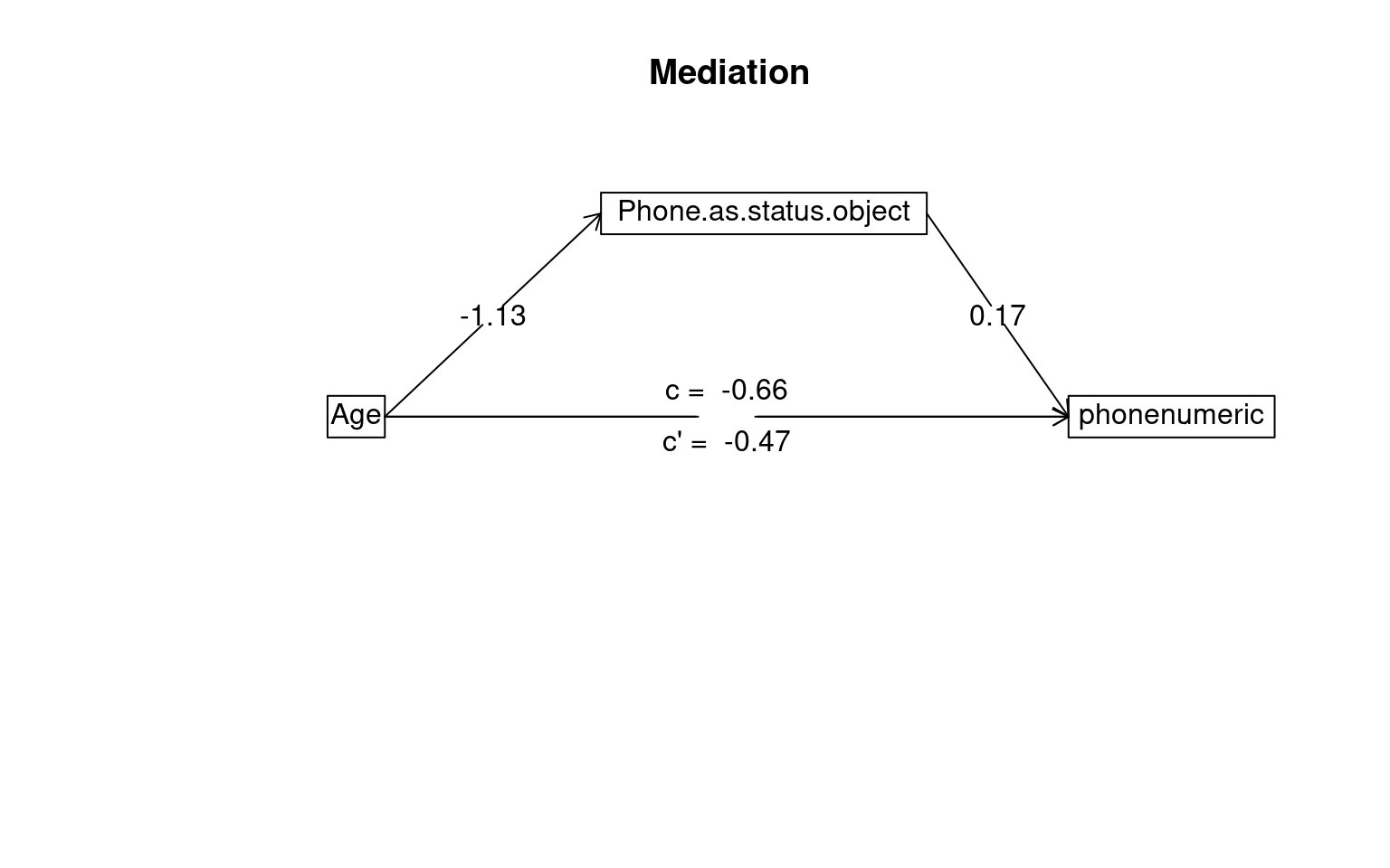
We can see that age and phone-as-status-symbol both correlate with iphone ownership. But are they independent? More importantly, can the effect of age be explained by the effect of status-symbol? I’ll rescale age to be between 0 and 1 to make the coefficients larger–otherwise this scaling doesn’t matter and unscaled age would produce the same results.
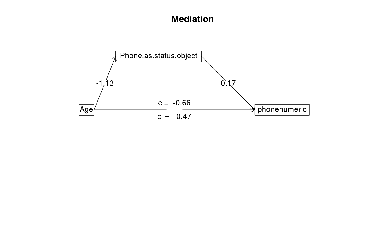
Mediation/Moderation Analysis
Call: psych::mediate(y = phonenumeric ~ Age + (Phone.as.status.object),
    data = dat)

The DV (Y) was  phonenumeric . The IV (X) was  Age . The mediating variable(s) =  Phone.as.status.object .

Total effect(c) of  Age  on  phonenumeric  =  -0.66   S.E. =  0.16  t  =  -4.06  df=  527   with p =  5.6e-05
Direct effect (c') of  Age  on  phonenumeric  removing  Phone.as.status.object  =  -0.47   S.E. =  0.17  t  =  -2.83  df=  526   with p =  0.0049
Indirect effect (ab) of  Age  on  phonenumeric  through  Phone.as.status.object   =  -0.2
Mean bootstrapped indirect effect =  -0.2  with standard error =  0.05  Lower CI =  -0.3    Upper CI =  -0.11
R = 0.27 R2 = 0.07   F = 20.29 on 2 and 526 DF   p-value:  1.87e-12

 To see the longer output, specify short = FALSE in the print statement or ask for the summary
The test suggests the indirect effect of age on phone usage through status symbol is statistically significant, but so is the direct effect. This suggests that although some of the impact of age on iphone usage can be explained by younger people being more likely to treat the phone as a status symbol (and those people tend to buy iphones), there is also a effect of age directly–even for people with the same level of phone-as-status-symbol, there is an age effect.
How about whether the relationship between gender and phone is mediated by emotionality?
Mediation/Moderation Analysis
Call: psych::mediate(y = phonenumeric ~ female + (Emotionality), data = dat)

The DV (Y) was  phonenumeric . The IV (X) was  female . The mediating variable(s) =  Emotionality .

Total effect(c) of  female  on  phonenumeric  =  0.2   S.E. =  0.05  t  =  4.34  df=  527   with p =  1.7e-05
Direct effect (c') of  female  on  phonenumeric  removing  Emotionality  =  0.15   S.E. =  0.05  t  =  3.01  df=  526   with p =  0.0028
Indirect effect (ab) of  female  on  phonenumeric  through  Emotionality   =  0.04
Mean bootstrapped indirect effect =  0.04  with standard error =  0.02  Lower CI =  0    Upper CI =  0.09
R = 0.2 R2 = 0.04   F = 11.42 on 2 and 526 DF   p-value:  2.88e-07

 To see the longer output, specify short = FALSE in the print statement or ask for the summary
Here, before we can tell if emotionality mediates the relationship between gender and phone, we need to know whether there IS a relationship. The mediate function first tests this, and finds it is significant. When emotionality is removed, the effect is still significant p=.0028. However, the indirect is also significant.
Exercise:
Form a mediation model for other variables within the iphone data.
Correspondence Analysis and Multiple Correspondence Analysis
Correspondance Analysis (CA) and Multiple Correspondence Analysis (MCA) are described as analogs to PCA for categorical variables. For example, it might be useful as an alternative to looking at cross-tabs for categorical variables. It can also be used in concert with inter-rater reliability to establish coding schemes that correspond with one another, or with k-means or other clustering to establish how different solutions correspond.
Resources
- Packages:
ca - corresp() in
MASS - https://www.utdallas.edu/~herve/Abdi-MCA2007-pretty.pdf
- http://gastonsanchez.com/visually-enforced/how-to/2012/10/13/MCA-in-R/
- Nenadic, O. and Greenacre, M. (2007). Correspondence analysis in R, with two- and three-dimensional graphics: The ca package. Journal of Statistical Software, 20 (3), http://www.jstatsoft.org/v20/i03/
Correspondence Analysis (CA) is available with the
corresp() in MASS and the ca package, which
provides better visualizations.
Background and Example
For CA, The basic problem we have is trying to understand whether two categorical variables have some sort of relationship. The problem is that, unless they are binary, correlation won’t work. One could imagine some sort of matching algorithm, to find how categories best align, and then finding the sum of the diagonals, but this gets tricky to pull off, especially if there is not a 1-1 mapping. Another problem is that we may not have the same number of levels of groups–can we come up with some sort of correspondence there? This is similar to the problem we face when looking at clustering solutions and trying to determine how well a solution corresponds to some particular category we used outside of the model. The clusters don’t have labels that will match the secondary variable, but we’d still like to measure how well they did.
Correspondence Analysis uses a PCA-style model to identify dimensions that the two categories correspond to, and maps category labels into that space.
To explore this, let’s start with the iris data, and k-means clustering, just to create an unlabeled set of groups that tends to correspond to our ground truth labeling.
library(MASS)
set.seed(5220)
iris2 <- scale(iris[, 1:4])
model <- kmeans(iris[, 1:4], centers = 3)

table(iris$Species, model$cluster)
              1  2  3
  setosa     50  0  0
  versicolor  0  2 48
  virginica   0 36 14
MASS library corresp function
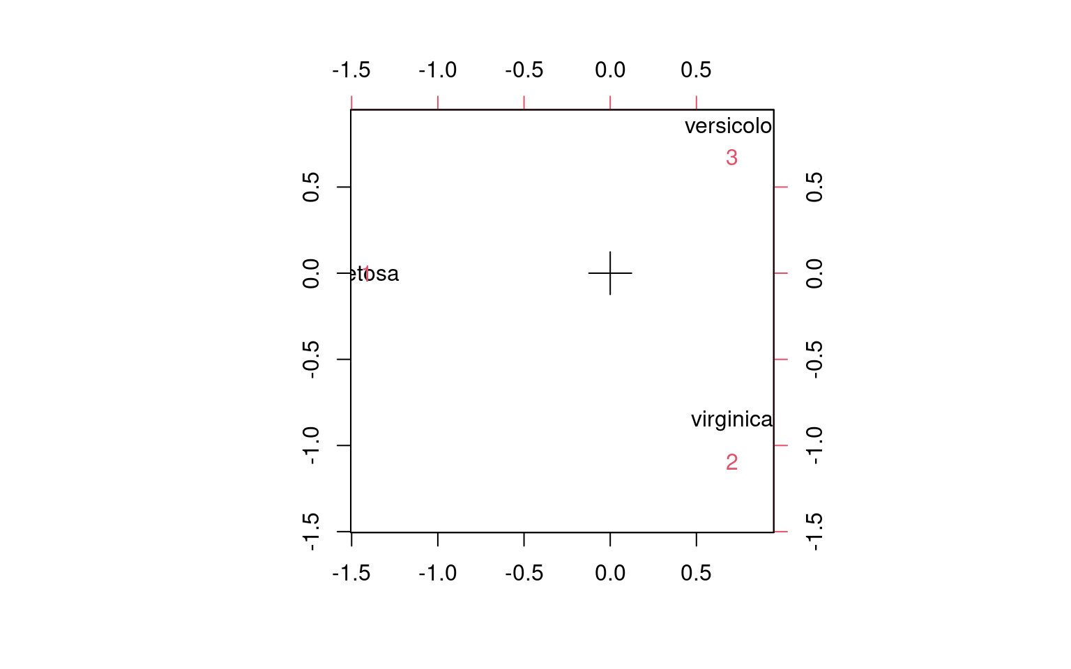
Can we measure how good the correspondence is between our clusters and the true species? The MASS library corresp implements CA, which takes as an argument the two sets of labels.
First canonical correlation(s): 1.0000000 0.7004728

 x scores:
                 [,1]          [,2]
setosa     -1.4142136  1.547367e-17
versicolor  0.7071068 -1.224745e+00
virginica   0.7071068  1.224745e+00

 y scores:
        [,1]          [,2]
1 -1.4142136  2.480643e-17
2  0.7071068  1.564407e+00
3 0.7071068 -9.588299e-01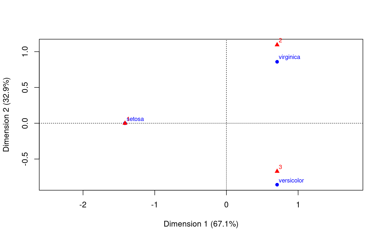 The two groups of three labels are each mapped into the same space,
which helps us recognize which match.
The two groups of three labels are each mapped into the same space,
which helps us recognize which match.
The model can also be specified in formula form. Here, we will make a 5-group k-means to see what that produces.
model <- kmeans(iris[, 1:4], centers = 5)
tmp <- data.frame(spec = iris$Species, cl = model$cluster)
camodel2 <- corresp(~spec + cl, data = tmp, nf = 2)
camodel2
First canonical correlation(s): 1.0000000 0.7004728
spec scores:
[,1] [,2]
setosa -1.4142136 1.840579e-16
versicolor 0.7071068 -1.224745e+00
virginica 0.7071068 1.224745e+00
cl scores:
[,1] [,2]
1 -1.4142136 -1.426398e-16
2 0.7071068 -9.588299e-01
3 -1.4142136 -4.999672e-17
4 0.7071068 1.564407e+00
5 -1.4142136 2.898980e-17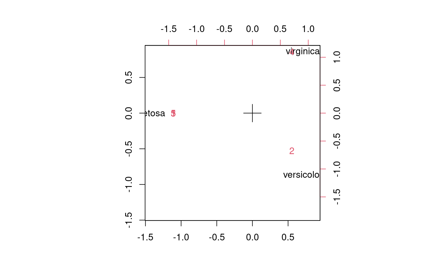 Not surprisingly, although the clusters break up into 5, these map
cleanly onto the 3 species they belong to.
Not surprisingly, although the clusters break up into 5, these map
cleanly onto the 3 species they belong to.
ca library ca function
A similar result can be obtained by doing ca on the cross-table.
 Principal inertias (eigenvalues):
           1      2
Value      1      0.490662
Percentage 67.08% 32.92%


 Rows:
           setosa versicolor virginica
Mass     0.333333   0.333333  0.333333
ChiDist  1.414214   1.111752  1.111752
Inertia  0.666667   0.411998  0.411998
Dim. 1  -1.414214   0.707107  0.707107
Dim. 2   0.000000  -1.224745  1.224745


 Columns:
                1         2         3        4         5
Mass     0.153333  0.413333  0.053333 0.253333  0.126667
ChiDist  1.414214  0.975240  1.414214 1.304159  1.414214
Inertia  0.306667  0.393118  0.106667 0.430877  0.253333
Dim. 1  -1.414214  0.707107 -1.414214 0.707107 -1.414214
Dim. 2   0.000000 -0.958830  0.000000 1.564407  0.000000
Principal inertias (eigenvalues):

 dim    value      %   cum%   scree plot
 1      10000000  67.1  67.1  *****************
 2      0.490662  32.9 100.0  ********
        -------- -----
 Total: 1.490662 100.0


Rows:
    name   mass  qlt  inr     k=1  cor ctr    k=2 cor ctr
1 | sets |  333 1000  447 | -1414 1000 667 |    0   0   0 |
2 | vrsc |  333 1000  276 |   707  405 167 | -858 595 500 |
3 | vrgn |  333 1000  276 |   707  405 167 |  858 595 500 |

Columns:
    name   mass  qlt  inr     k=1  cor ctr    k=2 cor ctr
1 |    1 |  153 1000  206 | -1414 1000 307 |    0   0   0 |
2 |    2 |  413 1000  264 |   707  526 207 | -672 474 380 |
3 |    3 |   53 1000   72 | -1414 1000 107 |    0   0   0 |
4 |    4 |  253 1000  289 |   707  294 127 | 1096 706 620 |
5 |    5 |  127 1000  170 | -1414 1000 253 |    0   0   0 |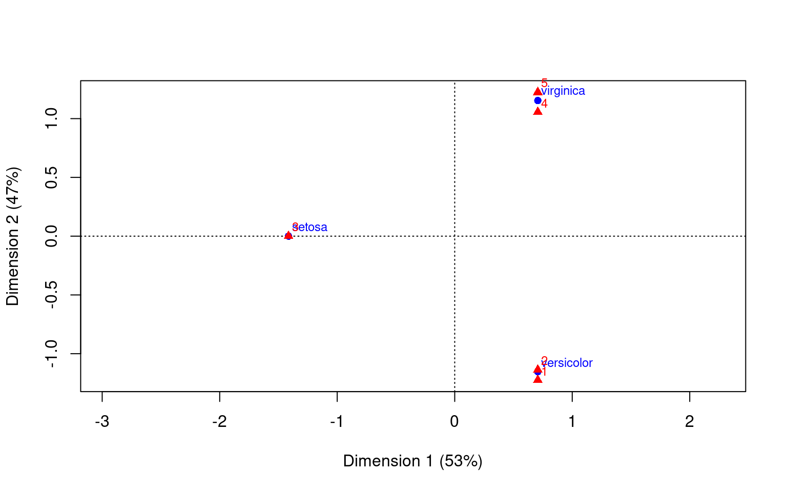
We can see that using any of these methods, we have mapped the categories into a space of principal components–technically using SVD. Furthermore it places both the ‘rows’ and ‘columns’ into that space, so we can see how closely aligned the groups are. We chose to use 2 dimensions in each case for easy visualization. So far, we used a data set with really strong correspondence. What if the correspondence is not as good?
set.seed(1001)
iris2 <- scale(iris[, 1:4])
model <- kmeans(iris[, 1:4], centers = 5)

table(iris$Species, model$cluster)
              1  2  3  4  5
  setosa      0  0 50  0  0
  versicolor 21 27  0  2  0
  virginica   0  1  0 27 22
 Principal inertias (eigenvalues):
           1   2
Value      1   0.886946
Percentage 53% 47%


 Rows:
           setosa versicolor virginica
Mass     0.333333   0.333333  0.333333
ChiDist  1.414214   1.352930  1.352930
Inertia  0.666667   0.610140  0.610140
Dim. 1  -1.414214   0.707107  0.707107
Dim. 2   0.000000  -1.224745  1.224745


 Columns:
                1         2         3        4        5
Mass     0.140000  0.186667  0.333333 0.193333 0.146667
ChiDist  1.414214  1.339167  1.414214 1.270726 1.414214
Inertia  0.280000  0.334762  0.666667 0.312184 0.293333
Dim. 1   0.707107  0.707107 -1.414214 0.707107 0.707107
Dim. 2 -1.300460 -1.207570 0.000000 1.121086 1.300460 This should match our intuition for where the two sets of labels
belong.
This should match our intuition for where the two sets of labels
belong.
Other Examples (from ca help file)
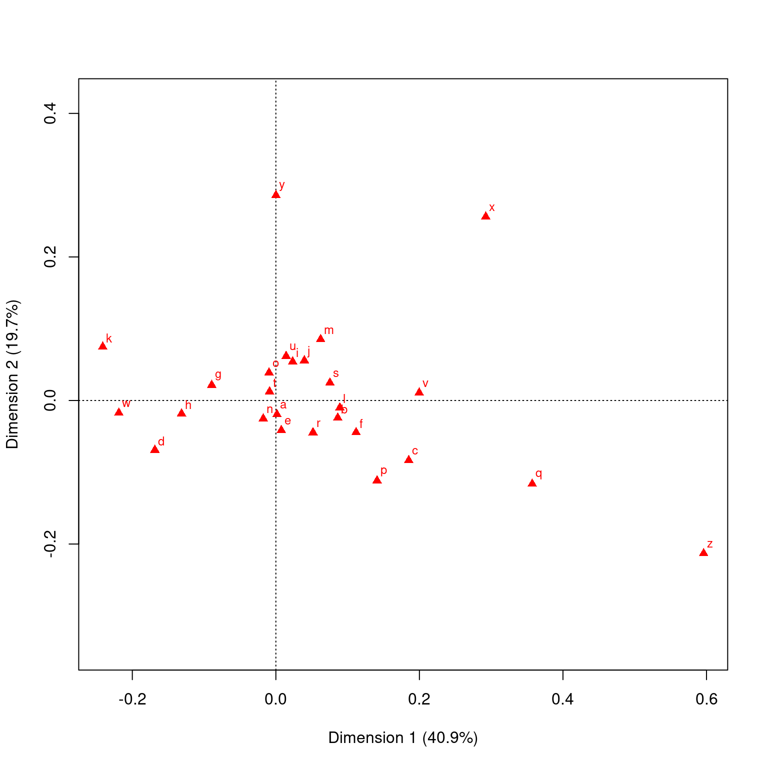
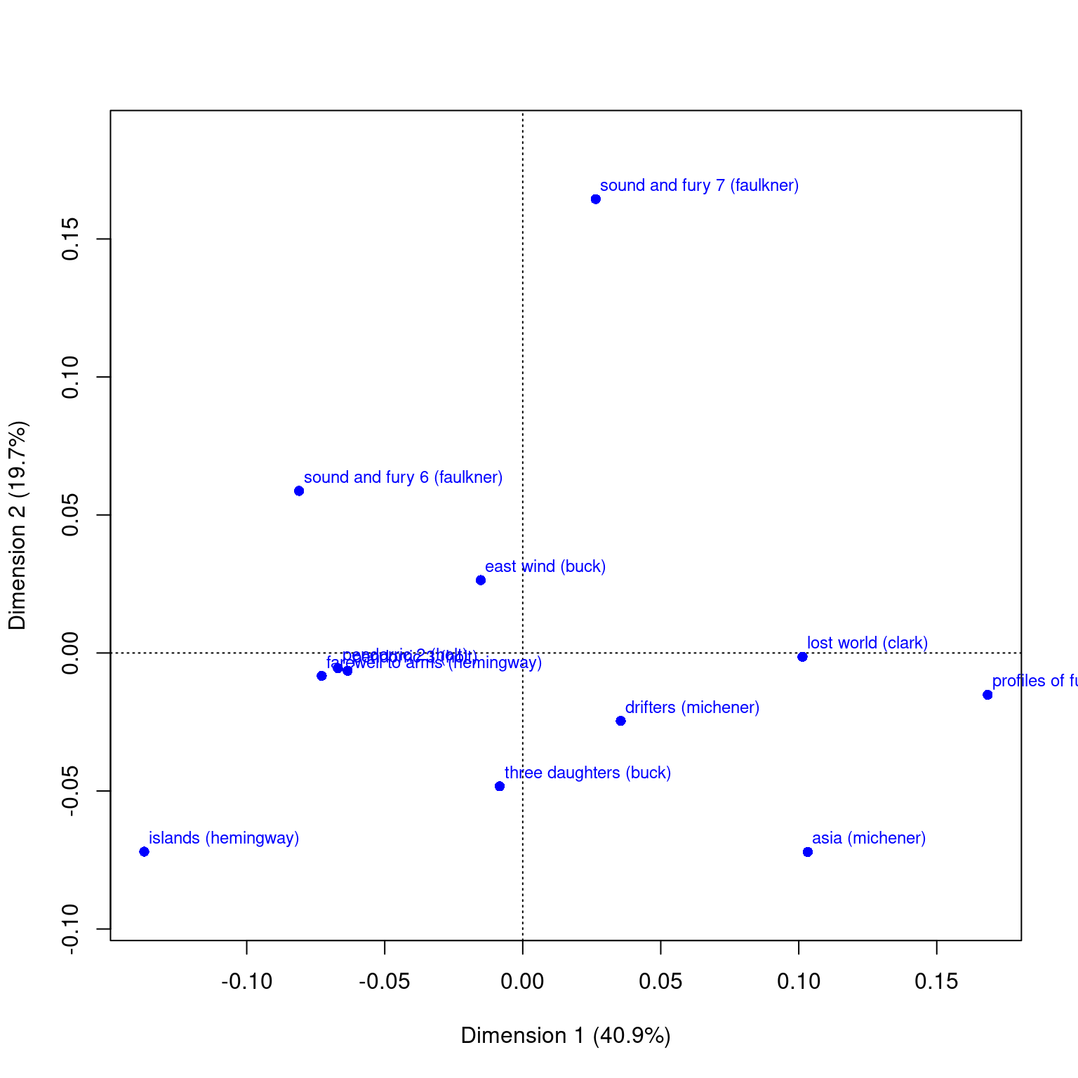
This data sets maps the distribution of letters of the alphabet to authors. These dimensions might be used to detect language, style, historic period, or something
 Principal inertias (eigenvalues):
           1        2        3        4        5        6        7
Value      0.007664 0.003688 0.002411 0.001383 0.001002 0.000723 0.000659
Percentage 40.91%   19.69%   12.87%   7.38%    5.35%    3.86%    3.52%
           8        9        10       11
Value      0.000455 0.000374 0.000263 0.000113
Percentage 2.43%    2%       1.4%     0.6%


 Rows:
        three daughters (buck) drifters (michener) lost world (clark)
Mass                  0.085407            0.079728           0.084881
ChiDist               0.097831            0.094815           0.128432
Inertia               0.000817            0.000717           0.001400
Dim. 1               -0.095388            0.405697           1.157803
Dim. 2               -0.794999           -0.405560          -0.023114
        east wind (buck) farewell to arms (hemingway)
Mass            0.089411                     0.082215
ChiDist         0.118655                     0.122889
Inertia         0.001259                     0.001242
Dim. 1         -0.173901                    -0.831886
Dim. 2          0.434443                    -0.136485
        sound and fury 7 (faulkner) sound and fury 6 (faulkner)
Mass                       0.082310                    0.083338
ChiDist                    0.172918                    0.141937
Inertia                    0.002461                    0.001679
Dim. 1                     0.302025                   -0.925572
Dim. 2                     2.707599                    0.966944
        profiles of future (clark) islands (hemingway) pendorric 3 (holt)
Mass                      0.089722            0.082776           0.079501
ChiDist                   0.187358            0.165529           0.113174
Inertia                   0.003150            0.002268           0.001018
Dim. 1                    1.924060           -1.566481          -0.724758
Dim. 2                   -0.249310           -1.185338          -0.106349
        asia (michener) pendorric 2 (holt)
Mass           0.077827           0.082884
ChiDist        0.155115           0.101369
Inertia        0.001873           0.000852
Dim. 1         1.179548          -0.764937
Dim. 2        -1.186934          -0.091188


 Columns:
                a         b         c         d         e         f         g
Mass     0.079847  0.015685  0.022798  0.045967  0.127070  0.019439  0.020025
ChiDist  0.048441  0.148142  0.222783  0.189938  0.070788  0.165442  0.156640
                h        i        j         k         l        m         n
Mass     0.064928 0.070092 0.000789  0.009181  0.042667 0.025500  0.068968
ChiDist  0.154745 0.086328 0.412075  0.296727  0.120397 0.159747  0.075706
                o         p         q         r        s         t        u
Mass     0.076572  0.015159  0.000669  0.051897 0.060660  0.093010 0.029756
ChiDist  0.088101  0.250617  0.582298  0.111725 0.123217  0.050630 0.119215
               v         w        x        y         z
Mass    0.009612  0.025847 0.001160 0.021902  0.000801
ChiDist 0.269770  0.232868 0.600831 0.301376  0.833700
 [ reached getOption("max.print") -- omitted 3 rows ]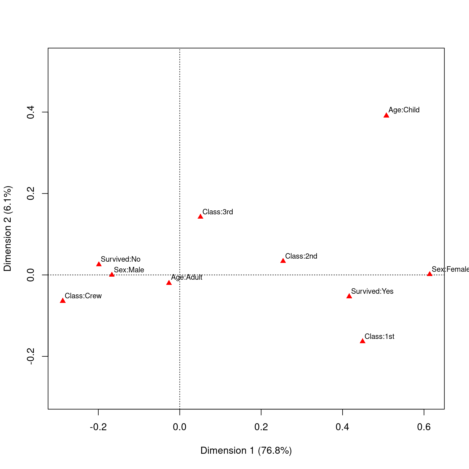
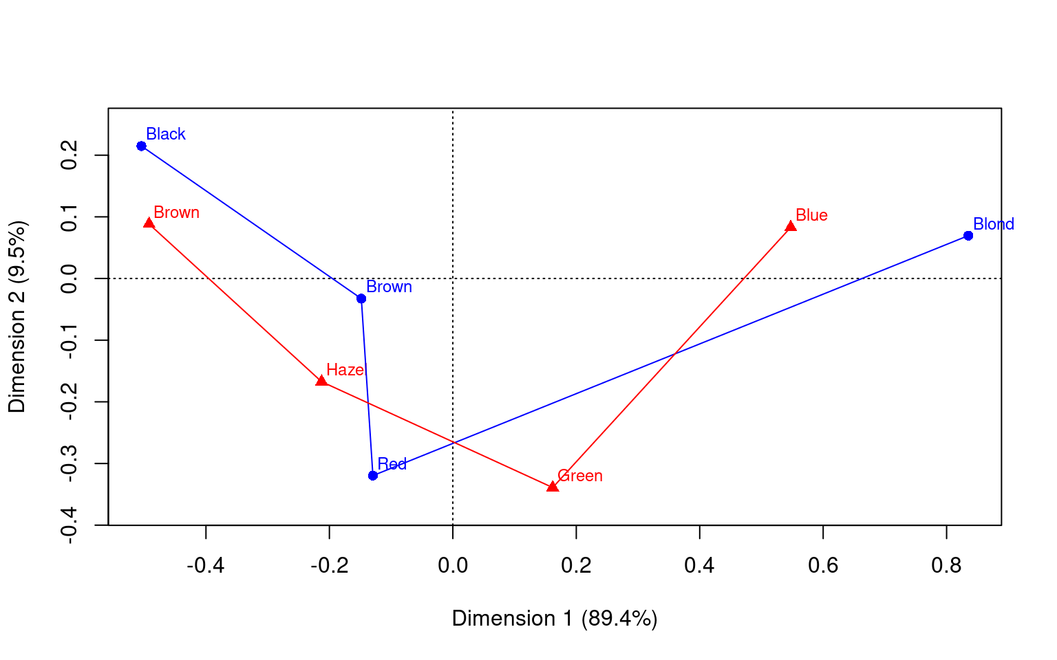
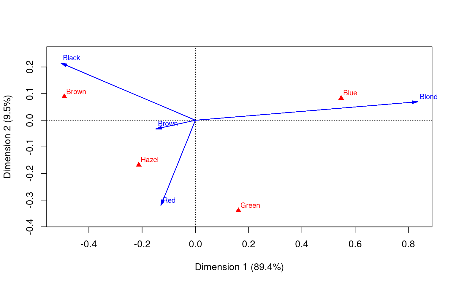
 Principal inertias (eigenvalues):
           1        2        3
Value      0.208773 0.022227 0.002598
Percentage 89.37%   9.52%    1.11%


 Rows:
            Black     Brown       Red    Blond
Mass     0.182432  0.483108  0.119932 0.214527
ChiDist  0.551192  0.159461  0.354770 0.838397
Inertia  0.055425  0.012284  0.015095 0.150793
Dim. 1  -1.104277 -0.324463 -0.283473 1.828229
Dim. 2   1.440917 -0.219111 -2.144015 0.466706


 Columns:
            Brown     Blue     Hazel     Green
Mass     0.371622 0.363176  0.157095  0.108108
ChiDist  0.500487 0.553684  0.288654  0.385727
Inertia  0.093086 0.111337  0.013089  0.016085
Dim. 1  -1.077128 1.198061 -0.465286  0.354011
Dim. 2   0.592420 0.556419 -1.122783 -2.274122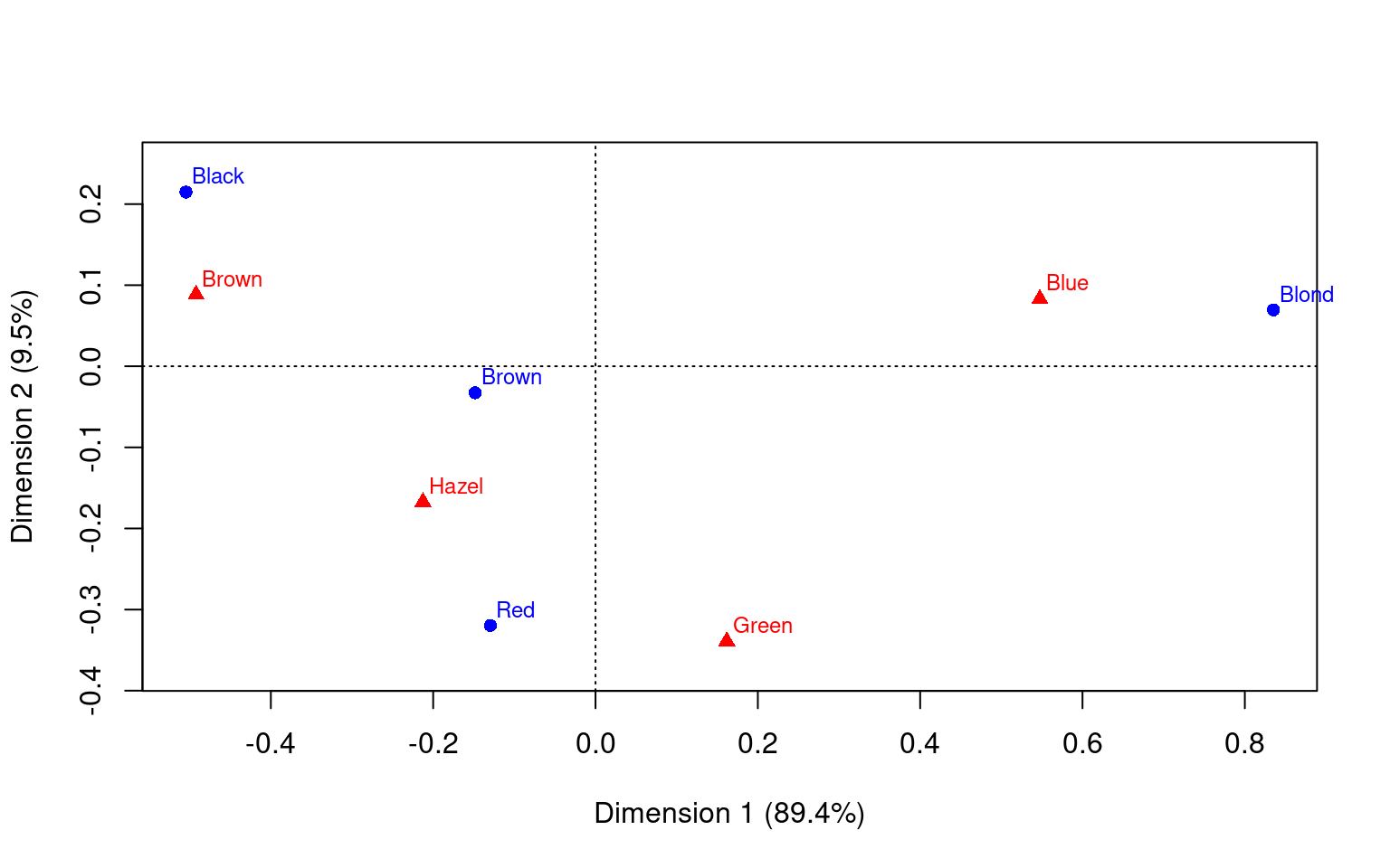
Multiple Correspondence Analysis
We have looked at a pair of variables, often as a contingency table, using CA. But what if you had a large number of measures that were all categorical–like a multiple-choice test. We could maybe adapt CA to tell us things more like factor analysis does for large-scale tests. In general, MCA will take the NxMxO contingency table and use SVD to map all the dimensions into a single space, showing you where the levels of each dimension fall. Let’s look at the Titanic survivor data set. Was it true that it was ‘women and children first?’ Who survived? Who didn’t?
, , Age = Child, Survived = No

      Sex
Class  Male Female
  1st     0      0
  2nd     0      0
  3rd    35     17
  Crew    0      0

, , Age = Adult, Survived = No

      Sex
Class  Male Female
  1st   118      4
  2nd   154     13
  3rd   387     89
  Crew  670      3

, , Age = Child, Survived = Yes

      Sex
Class  Male Female
  1st     5      1
  2nd    11     13
  3rd    13     14
  Crew    0      0

, , Age = Adult, Survived = Yes

      Sex
Class  Male Female
  1st    57    140
  2nd    14     80
  3rd    75     76
  Crew  192     20
 Eigenvalues:
           1        2        3
Value      0.067655 0.005386 0
Percentage 76.78%   6.11%    0%


 Columns:
        Class:1st Class:2nd Class:3rd Class:Crew Sex:Female  Sex:Male Age:Adult
Mass     0.036915  0.032372  0.080191   0.100522   0.053385  0.196615  0.237619
ChiDist  1.277781  1.316778  0.749611   0.667164   1.126763  0.305938  0.118369
Inertia  0.060272  0.056129  0.045061   0.044743   0.067777  0.018403  0.003329
Dim. 1  -1.726678 -0.976191 -0.195759   1.104622  -2.360505  0.640923  0.101670
Dim. 2  -2.229588  0.457212  1.937417  -0.874018   0.016164 -0.004389 -0.277601
        Age:Child Survived:No Survived:Yes
Mass     0.012381    0.169241     0.080759
ChiDist  2.271810    0.394352     0.826420
Inertia  0.063898    0.026319     0.055156
Dim. 1  -1.951309    0.763670    -1.600378
Dim. 2   5.327911    0.344441    -0.721825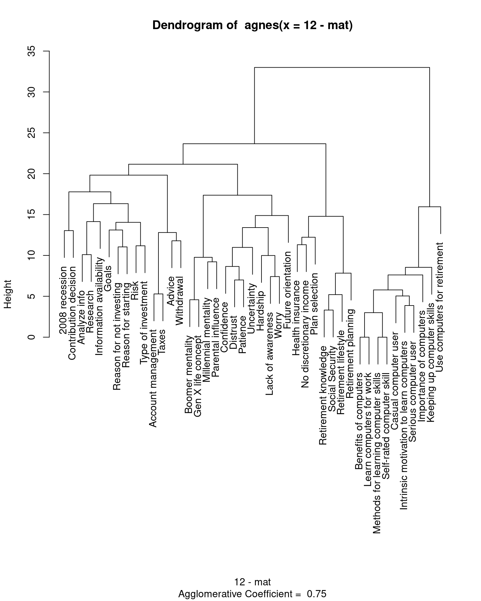
This shows two locations for survival. The different marginal groups cluster closer to one or another of these in ways we probably expect. Adult men and crew members (probably also mostly adult men) were likely to not survive.
Application: Card-sorting and survey data
The following data set involves a card-sort exercise, which is a common way of understanding users mental models. In this data set collected by Natasha Hardy as part of her dissertation at MTU, A set of 43 topics related to financial planning for retirement were sorted into groups by participants. Each participant could form any group they wanted, and then groups were labelled–but each participant may have used a different sorting. Let’s first look at these as a dissimilarity measure and do some clustering and MDS plotting.
library(MASS)
data <- read.csv("natasha_data.csv")
tab1 <- table(data$participant, data$card.label, data$category.label)

mat <- matrix(0, dim(tab1)[2], dim(tab1)[2])
rownames(mat) <- colnames(mat) <- rownames(tab1[1, , ])
for (sub in 1:dim(tab1)[1]) {

    t1 <- tab1[sub, , ]
    byindex <- apply(t1, 1, function(x) {
        which(x == 1)
    })
    submat <- outer(byindex, byindex, "==")
    mat <- mat + submat

}
rownames(mat)
[1] "2008 recession"
[2] "Account management"
[3] "Advice"
[4] "Analyze info"
[5] "Benefits of computers"
[6] "Boomer mentality"
[7] "Casual computer user"
[8] "Confidence"
[9] "Contribution decision"
[10] "Distrust"
[11] "Future orientation"
[12] "Gen X life concept"
[13] "Goals"
[14] "Hardship"
[15] "Health insurance"
[16] "Importance of computers"
[17] "Information availability"
[18] "Intrinsic motivation to learn computers"
[19] "Keeping up computer skills"
[20] "Lack of awareness"
[21] "Learn computers for work"
[22] "Methods for learning computer skills"
[23] "Millennial mentality"
[24] "No discretionary income"
[25] "Parental influence"
[26] "Patience"
[27] "Plan selection"
[28] "Reason for not investing"
[29] "Reason for starting"
[30] "Research"
[31] "Retirement knowledge"
[32] "Retirement lifestyle"
[33] "Retirement planning"
[34] "Risk"
[35] "Self-rated computer skill"
[36] "Serious computer user"
[37] "Social Security"
[38] "Taxes"
[39] "Type of investment"
[40] "Uncertainty"
[41] "Use computers for retirement"
[42] "Withdrawal"
[43] "Worry" 
K-means cluster
                         2008 recession                      Account management
                                      2                                       2
                                 Advice                            Analyze info
                                      2                                       2
                  Benefits of computers                        Boomer mentality
                                      3                                       4
                   Casual computer user                              Confidence
                                      3                                       4
                  Contribution decision                                Distrust
                                      1                                       4
                     Future orientation                      Gen X life concept
                                      4                                       4
                                  Goals                                Hardship
                                      2                                       4
                       Health insurance                 Importance of computers
                                      1                                       3
               Information availability Intrinsic motivation to learn computers
                                      2                                       3
             Keeping up computer skills                       Lack of awareness
                                      3                                       4
               Learn computers for work    Methods for learning computer skills
                                      3                                       3
                   Millennial mentality                 No discretionary income
                                      4                                       1
                     Parental influence                                Patience
                                      4                                       4
                         Plan selection                Reason for not investing
                                      1                                       2
                    Reason for starting                                Research
                                      2                                       2
                   Retirement knowledge                    Retirement lifestyle
                                      1                                       1
                    Retirement planning                                    Risk
                                      1                                       2
              Self-rated computer skill                   Serious computer user
                                      3                                       3
                        Social Security                                   Taxes
                                      1                                       2
                     Type of investment                             Uncertainty
                                      2                                       4
           Use computers for retirement                              Withdrawal
                                      3                                       2
                                  Worry
4 initial value 31.345692
final value 31.345692
convergedplot(mds$points[, 1], mds$points[, 2], type = "n")
text(mds$points[, 1], mds$points[, 2], rownames(mat), col = km$cluster)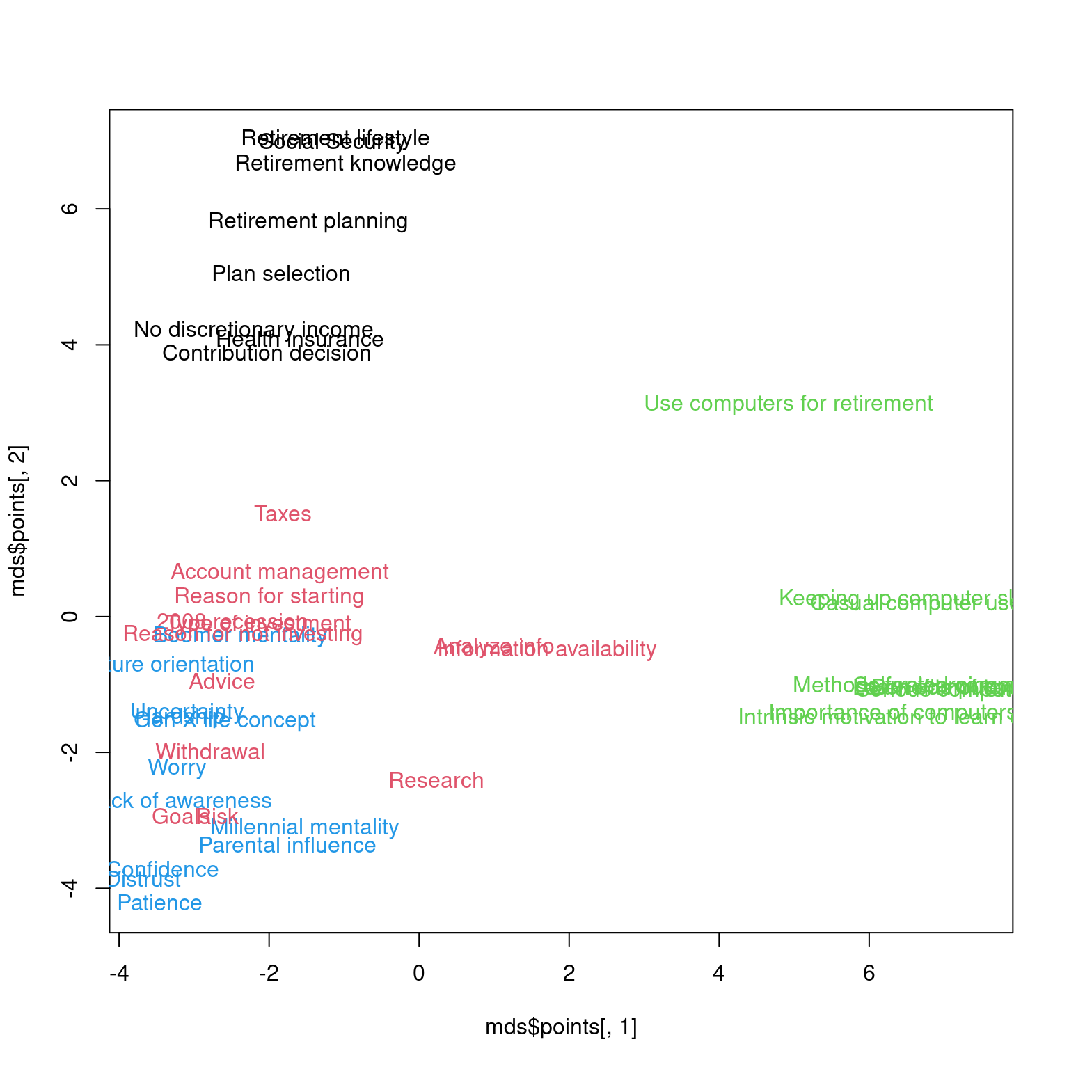
Correspondence analysis
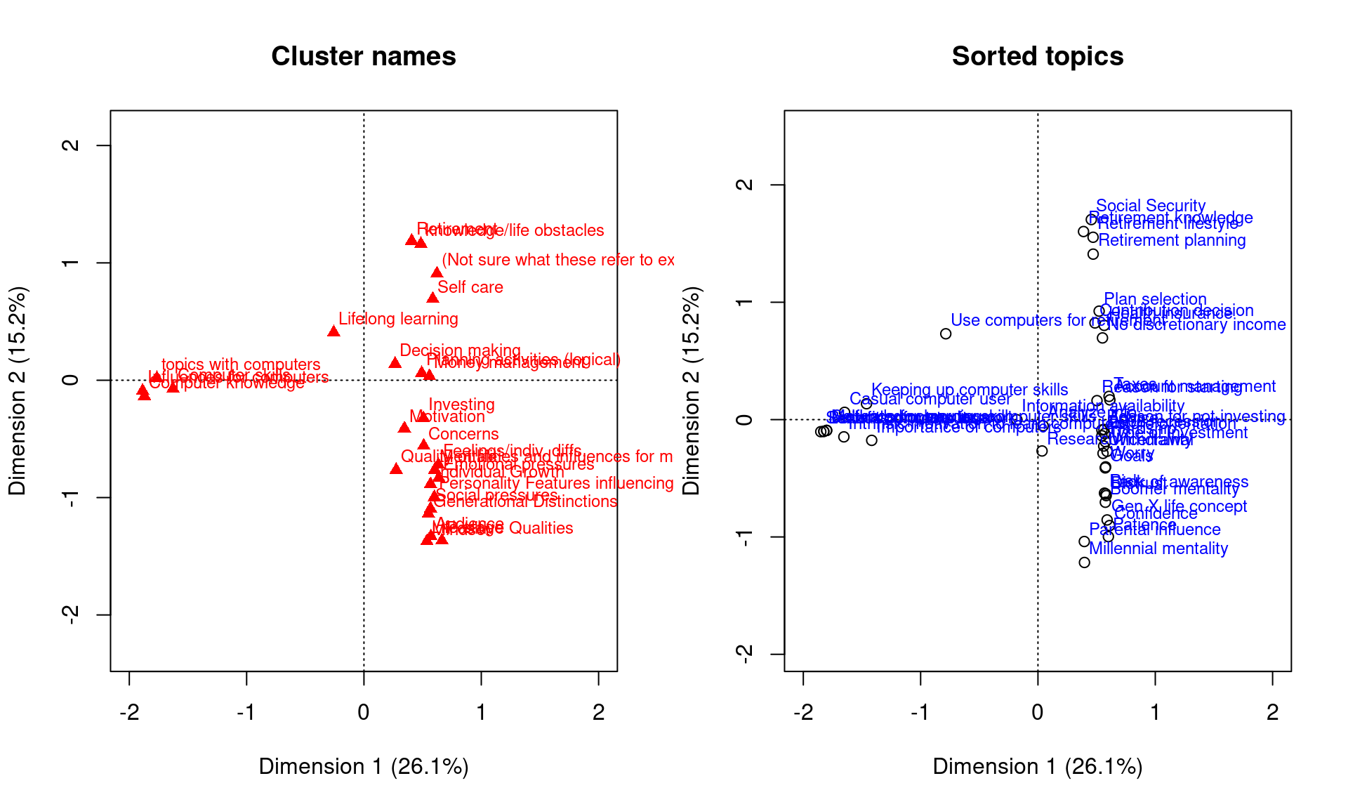
Because each participant labeled the groupings, we can also do a CA. Here, two levels of variables will have some correspondence, and we can use CA to map these into a common vector space.
library(ca)
ca <- ca(table(as.factor(data$card.label), as.factor(data$category.label)))
plot(ca, arrows = c(F, T), xlim = c(-2, 2))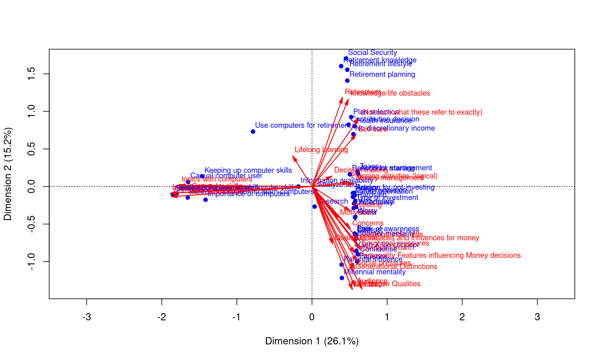
par(mfrow = c(1, 2))

plot.ca(ca, dim = c(1, 2), what = c("none", "all"), main = "Cluster names", xlim = c(-2,
    2))
# points(ca$rowcoord[,1], ca$rowcoord[,2],col=km$cluster,pch=16)

plot(ca, dim = c(1, 2), what = c("all", "none"), main = "Sorted topics", xlim = c(-2,
    2), col = c("black", "orange"), pch = 1)