Generalized Additive Models (GAMs)
Generalized Additive Models (GAMs)
Generalized Additive Models (GAMs) are an advance over glms that allow you to integrate and combine transformations of the input variables, including things like lowess smoothing. The basic approach is framed similar to a glm, but we can specify transforms within the syntax of the model, these transforms get applied optimally to predict the outcome, and then look at the transformed relationship as part of the model.
A GAM is essentially a regression model, but the gam library permits glms and mixed effects models as well. A binomial glm is logistic regression and essentially a classifier, so it is easy to generalize.
GAMs have been around since the 1990s, but have recently come into resurgence as a means of developing more interpretable models. The flexibility of having numerous input transforms gives them a lot of potential predictive power that simpler regression models do not have, but the ability to trace the link makes them easier to understand than something like SVMs.
Libraries used:
gam
Let’s first look at the iphone data set. The gam library works best with numeric predictors and outcomes, so we will do some transformations first:
library(gam)
iphone <- read.csv("data_study1.csv")
values <- iphone[, -1]
values$phone <- 0 + (iphone$Smartphone == "iPhone")  ## Convert to a 0/1 number
values$Gender <- 0 + (values$Gender == "female")  #convert to a number
A basic GAM model
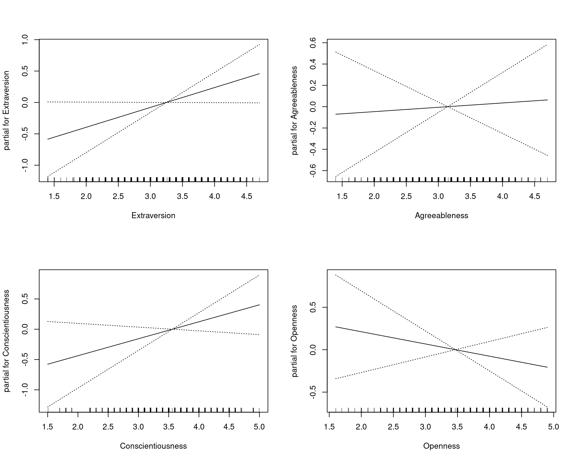
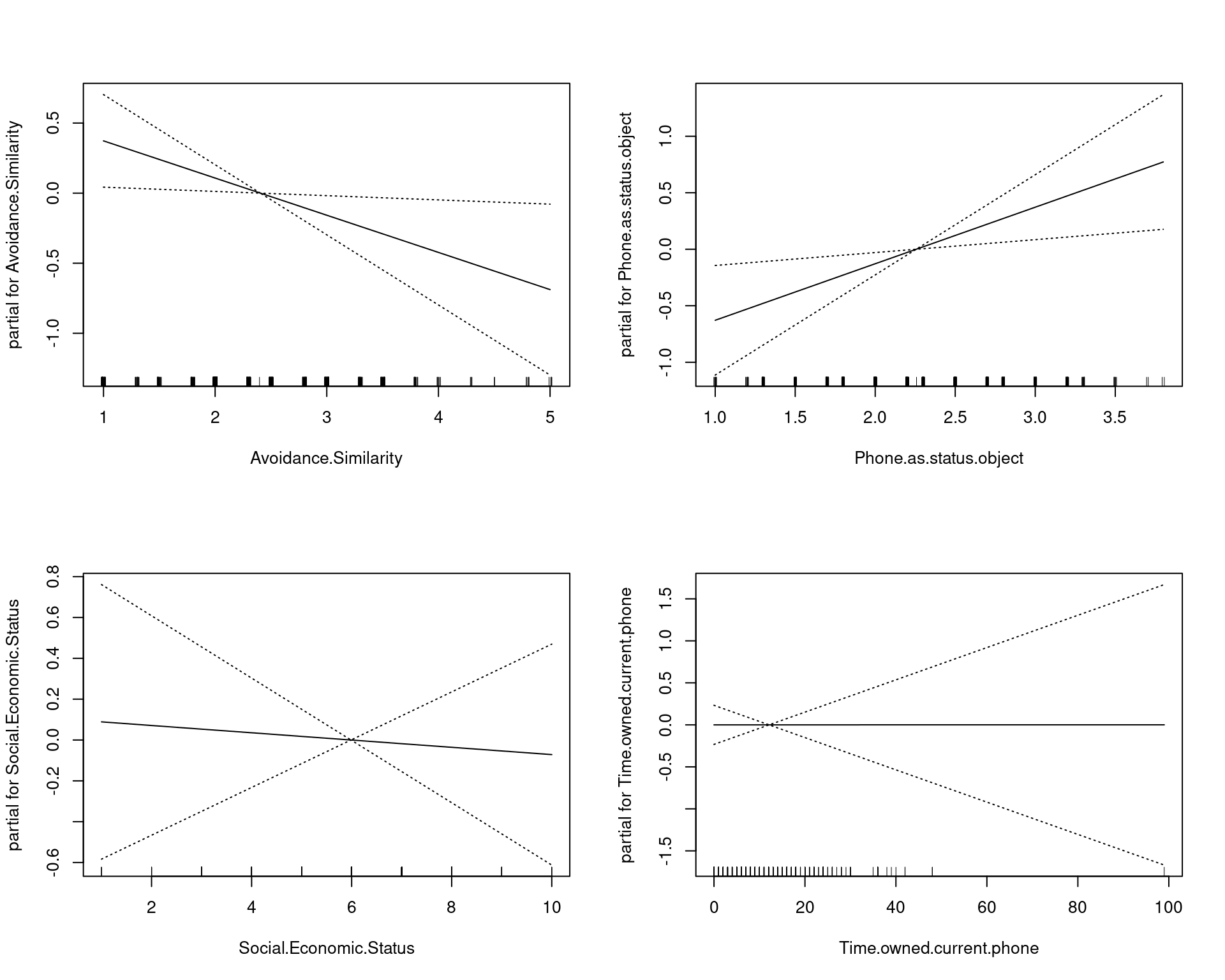
A simple GAM looks basically like a glm. We can see that initially, the model gets 69% accuracy, which is about as good as any of the classifiers we developed were (of course, we would worry about cross-validation). One thing the gam library does is plot the relationship between each predictor and the outcome. In this case, they are all linear predictors. This visualization is important because it lets us assess individual relationships.
library(DAAG)
model <- gam(phone ~ ., data = values, family = "binomial", trace = T)
GAM lm.wfit loop 1: deviance = 644.3867
GAM lm.wfit loop 2: deviance = 644.1742
GAM lm.wfit loop 3: deviance = 644.1741 confusion(predict(model) > 0, iphone$Smartphone)Overall accuracy = 0.69
Confusion matrix
Predicted (cv)
Actual [,1] [,2]
[1,] 0.659 0.341
[2,] 0.295 0.705predict(model, type = "terms") Gender Age Honesty.Humility Emotionality Extraversion
1 -0.4313575 0.067792521 0.08412966 -0.157058567 0.01565584
2 -0.4313575 -0.146609095 -0.02521823 -0.124444639 0.33176044
3 -0.4313575 -0.032261566 -0.24391399 -0.157058567 -0.17400691
4 -0.4313575 0.096379403 0.24815148 -0.059216782 -0.14239646
5 -0.4313575 -0.203782859 -0.07989217 -0.254900351 -0.39528013
6 -0.4313575 0.082085962 0.46684724 0.103852858 -0.07917554
Agreeableness Conscientiousness Openness Avoidance.Similarity
1 0.010378617 -0.12933283 0.024267499 0.37281830
2 0.034797986 -0.10131601 -0.148628215 0.37281830
3 0.038867881 0.03876807 -0.206260119 -0.15777325
4 -0.030320332 -0.38148418 0.139531307 0.10752252
5 -0.022180543 0.09480170 0.053083451 -0.15777325
6 -0.030320332 0.09480170 -0.047772382 0.10752252
Phone.as.status.object Social.Economic.Status Time.owned.current.phone
1 -0.22817602 -0.0002356747 2.383193e-05
2 -0.12808886 -0.0180459500 -4.092360e-05
3 -0.47839392 0.0710054266 4.002082e-05
4 0.22221620 0.0353848759 -4.092360e-05
5 -0.52843750 0.0531951512 -3.282916e-05
6 -0.27821960 -0.0002356747 4.406804e-05
[ reached getOption("max.print") -- omitted 523 rows ]
attr(,"constant")
[1] 0.3985957par(mfrow = c(2, 2))
plot(model, se = TRUE)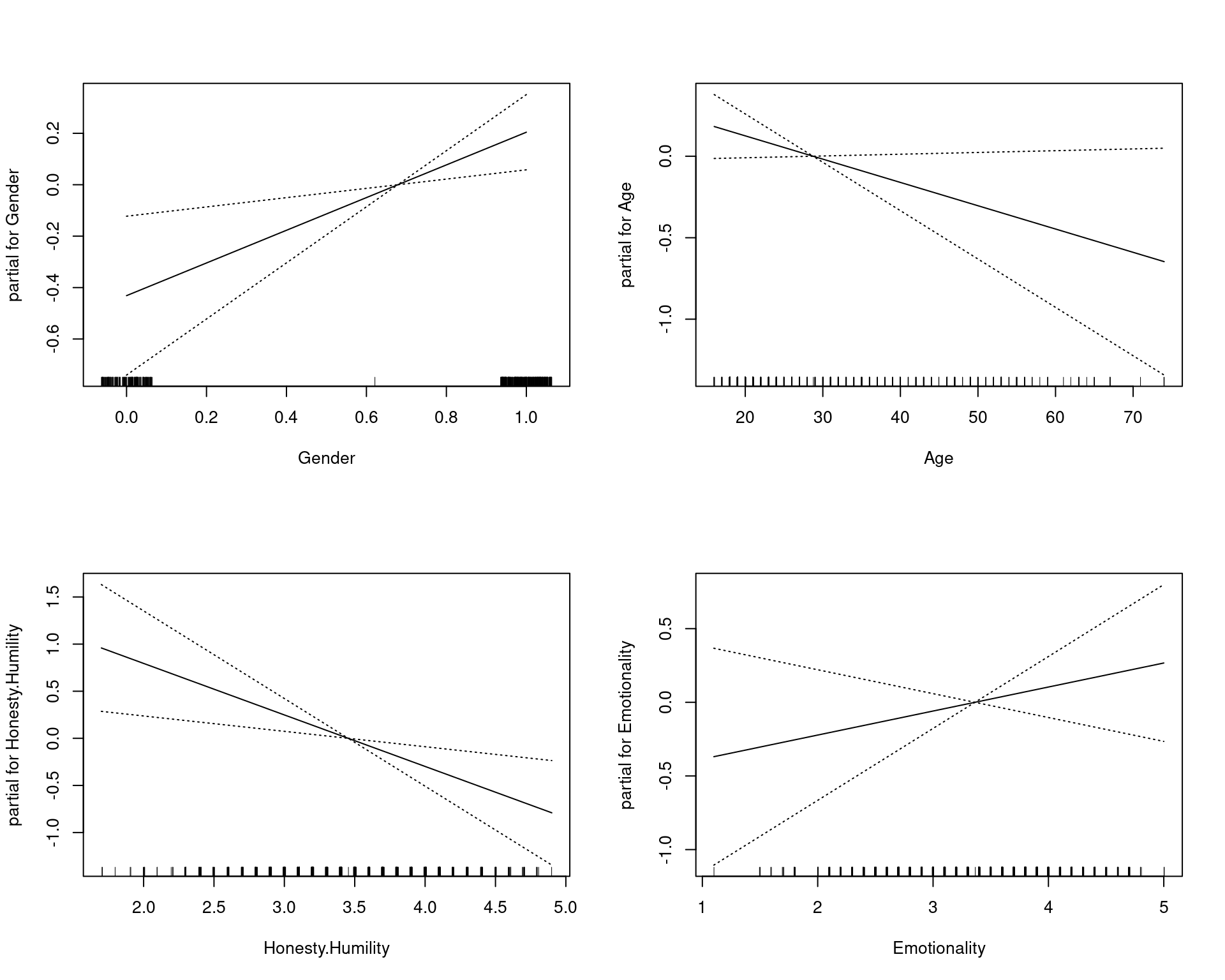
summary(model)
Call: gam(formula = phone ~ ., family = "binomial", data = values,
    trace = T)
Deviance Residuals:
    Min      1Q  Median      3Q     Max
-2.2383 -1.0875  0.6497  0.9718  1.8392

(Dispersion Parameter for binomial family taken to be 1)

    Null Deviance: 717.6175 on 528 degrees of freedom
Residual Deviance: 644.1741 on 516 degrees of freedom
AIC: 670.1741

Number of Local Scoring Iterations: 3

Anova for Parametric Effects
                          Df Sum Sq Mean Sq F value    Pr(>F)
Gender                     1  13.51 13.5102 12.9938 0.0003428 ***
Age                        1  11.00 10.9998 10.5794 0.0012184 **
Honesty.Humility           1  13.33 13.3340 12.8244 0.0003745 ***
Emotionality               1   2.00  1.9993  1.9229 0.1661355
Extraversion               1   4.70  4.7002  4.5205 0.0339643 *
Agreeableness              1   0.20  0.1950  0.1876 0.6651349
Conscientiousness          1   1.80  1.7985  1.7297 0.1890294
Openness                   1   2.24  2.2434  2.1576 0.1424739
Avoidance.Similarity       1   5.85  5.8526  5.6289 0.0180326 *
Phone.as.status.object     1   6.81  6.8089  6.5487 0.0107804 *
Social.Economic.Status     1   0.07  0.0701  0.0674 0.7952801
Time.owned.current.phone   1   0.00  0.0000  0.0000 0.9996705
 [ reached getOption("max.print") -- omitted 1 row ]
---
Signif. codes:  0 '***' 0.001 '**' 0.01 '*' 0.05 '.' 0.1 ' ' 1
The summary() function conducts a basic ANOVA table. Based on this, we might want to select a smaller set of variables
model2 <- gam(phone ~ Age + Honesty.Humility + Extraversion + Emotionality + Avoidance.Similarity +
    Phone.as.status.object + Social.Economic.Status, data = values, family = "binomial",
    trace = T)
GAM lm.wfit loop 1: deviance = 656.706
GAM lm.wfit loop 2: deviance = 656.4687
GAM lm.wfit loop 3: deviance = 656.4687
GAM lm.wfit loop 4: deviance = 656.4687 confusion(predict(model2) > 0, iphone$Smartphone)Overall accuracy = 0.669
Confusion matrix
Predicted (cv)
Actual [,1] [,2]
[1,] 0.634 0.366
[2,] 0.315 0.685par(mfrow = c(2, 2))
plot(model2, se = TRUE)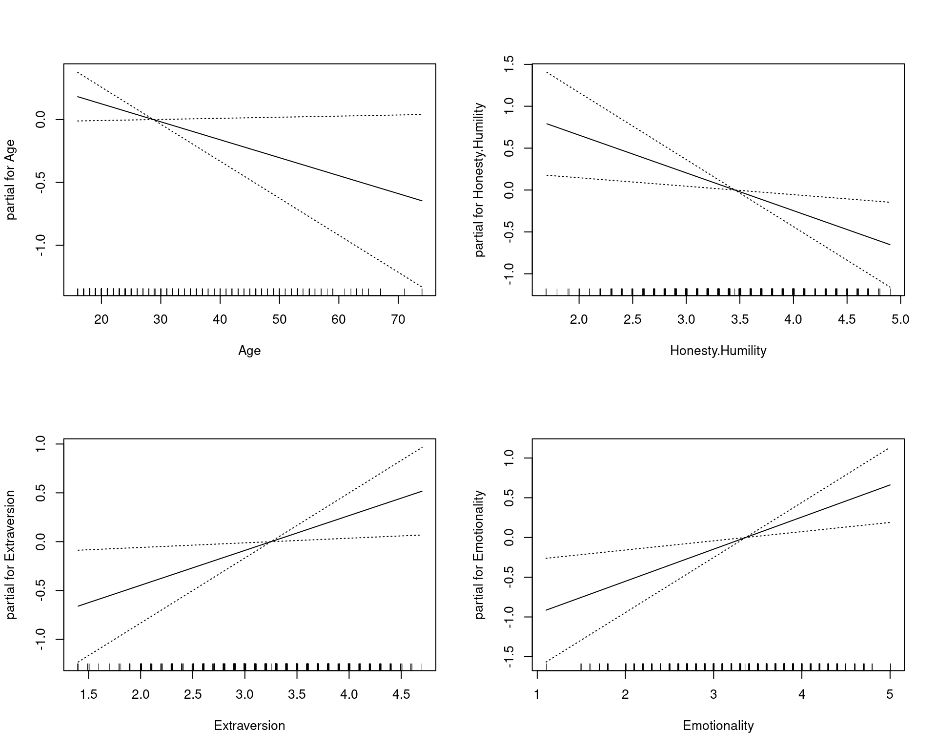
summary(model2)
Call: gam(formula = phone ~ Age + Honesty.Humility + Extraversion +
    Emotionality + Avoidance.Similarity + Phone.as.status.object +
    Social.Economic.Status, family = "binomial", data = values,
    trace = T)
Deviance Residuals:
    Min      1Q  Median      3Q     Max
-1.9925 -1.1346  0.6809  0.9803  1.9695

(Dispersion Parameter for binomial family taken to be 1)

    Null Deviance: 717.6175 on 528 degrees of freedom
Residual Deviance: 656.4687 on 521 degrees of freedom
AIC: 672.4687

Number of Local Scoring Iterations: 4

Anova for Parametric Effects
                        Df Sum Sq Mean Sq F value    Pr(>F)
Age                      1  11.94 11.9419 11.7262 0.0006648 ***
Honesty.Humility         1  10.74 10.7416 10.5476 0.0012383 **
Extraversion             1   3.66  3.6587  3.5927 0.0585887 .
Emotionality             1  11.99 11.9886 11.7721 0.0006490 ***
Avoidance.Similarity     1   6.61  6.6122  6.4928 0.0111171 *
Phone.as.status.object   1   6.96  6.9596  6.8339 0.0092032 **
Social.Economic.Status   1   0.01  0.0091  0.0089 0.9248144
Residuals              521 530.58  1.0184
---
Signif. codes:  0 '***' 0.001 '**' 0.01 '*' 0.05 '.' 0.1 ' ' 1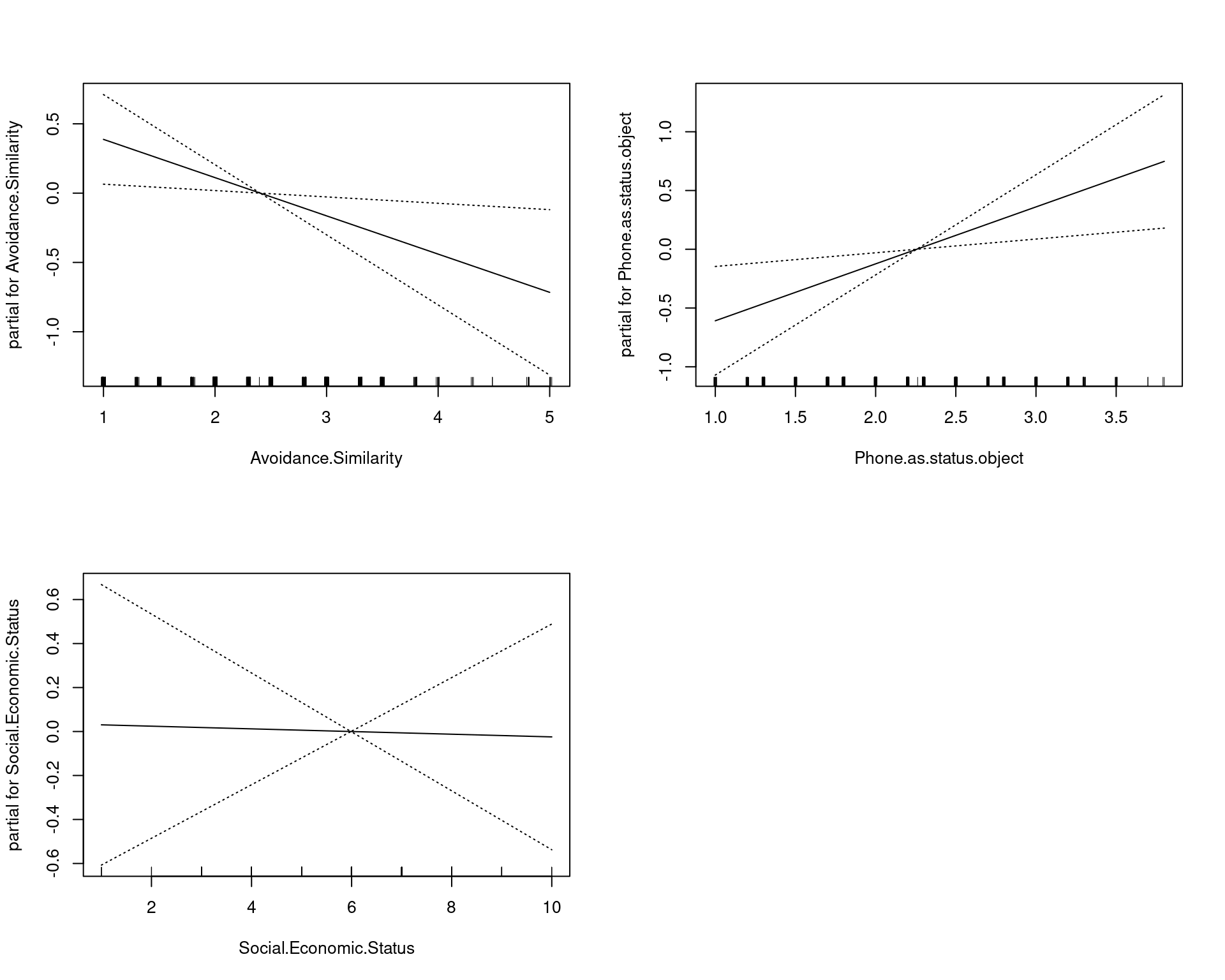
Accuracy suffers for the smaller model a little bit, but hopefully we are going to have a more general model that does not overfit.
Incorporating transforms into a GAM
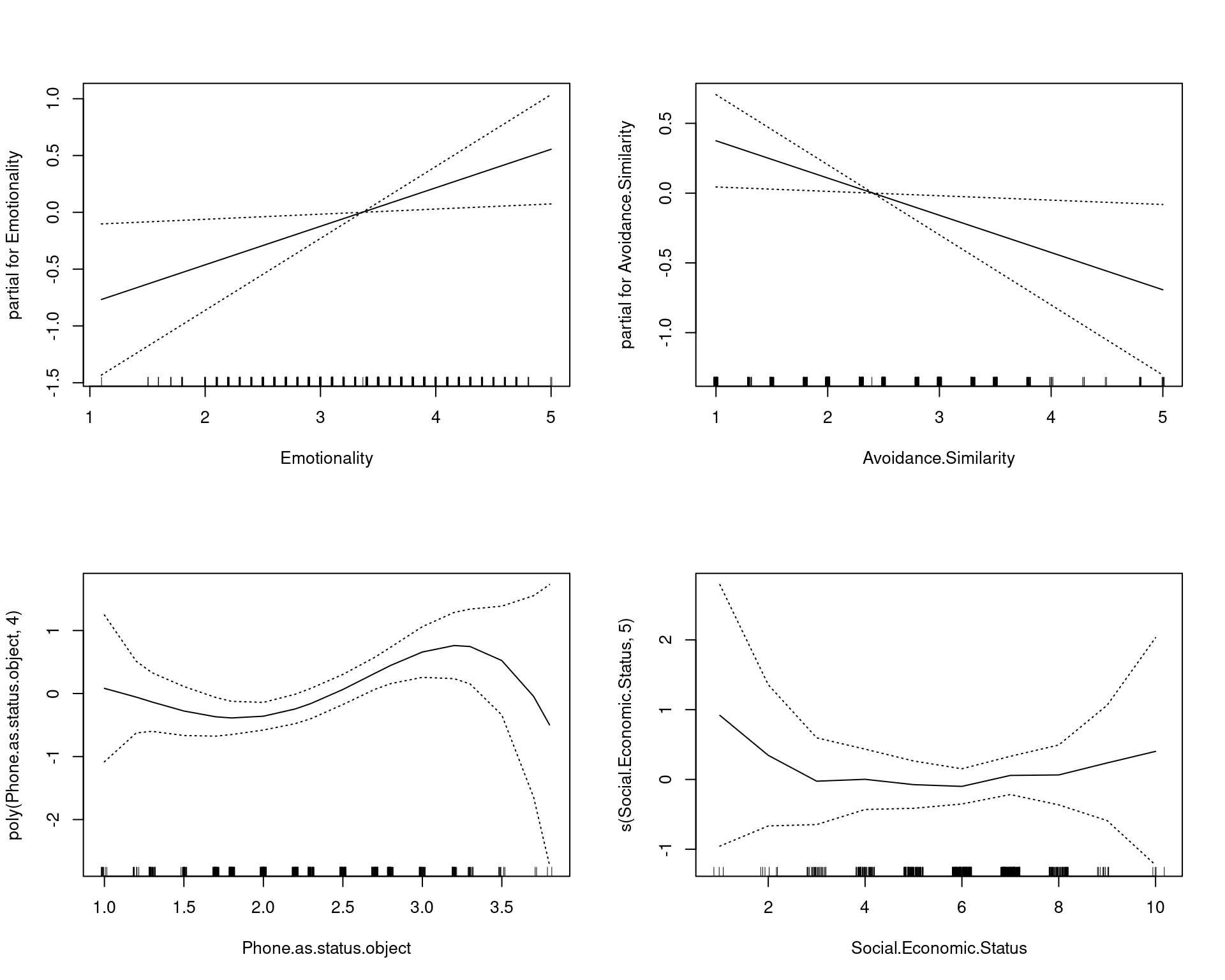
The advantage of a GAM is that we can specify various transforms within the predictor set, such as poly(), log(), and s()–which is a loess-style smoothing function. s(variable,n) will permit a smoothing function with 4 degrees of freedom–sort of a polynomial of the 4th order. Let’s try this with two of the strongest predictors. We will add a 4th-order smoothed function of age, and a polynomial of phone-as-status, and a smoothed function of SES, which we might suspect could be non-linear.
model3 <- gam(phone ~ Age + s(Age, 4) + Honesty.Humility + Extraversion + Emotionality +
    Avoidance.Similarity + poly(Phone.as.status.object, 4) + s(Social.Economic.Status,
    5), data = values, family = "binomial", trace = T)
GAM s.wam loop 1: deviance = 629.5864
GAM s.wam loop 2: deviance = 630.1319
GAM s.wam loop 3: deviance = 630.1627
GAM s.wam loop 4: deviance = 630.1626
GAM s.wam loop 5: deviance = 630.1626 confusion(predict(model3) > 0, iphone$Smartphone)Overall accuracy = 0.694
Confusion matrix
Predicted (cv)
Actual [,1] [,2]
[1,] 0.652 0.348
[2,] 0.284 0.716par(mfrow = c(2, 2))
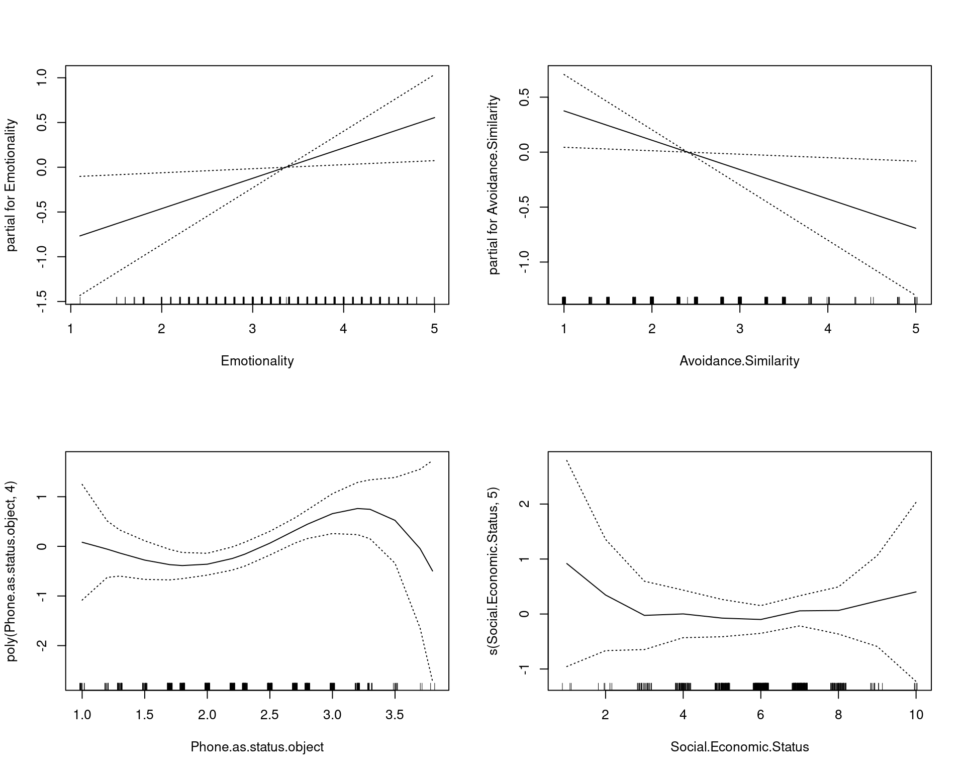
plot(model3, se = TRUE)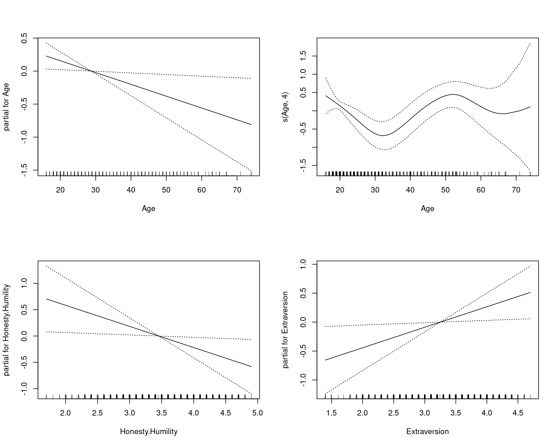
summary(model3)
Call: gam(formula = phone ~ Age + s(Age, 4) + Honesty.Humility + Extraversion +
    Emotionality + Avoidance.Similarity + poly(Phone.as.status.object,
    4) + s(Social.Economic.Status, 5), family = "binomial", data = values,
    trace = T)
Deviance Residuals:
    Min      1Q  Median      3Q     Max
-2.0999 -1.0671  0.6010  0.9798  1.7414

(Dispersion Parameter for binomial family taken to be 1)

    Null Deviance: 717.6175 on 528 degrees of freedom
Residual Deviance: 630.1626 on 511.0002 degrees of freedom
AIC: 666.1621

Number of Local Scoring Iterations: NA

Anova for Parametric Effects
                                 Df Sum Sq Mean Sq F value    Pr(>F)
Age                               1  12.42 12.4229 12.3224 0.0004871 ***
Honesty.Humility                  1   9.25  9.2499  9.1751 0.0025775 **
Extraversion                      1   4.24  4.2412  4.2069 0.0407693 *
Emotionality                      1   9.32  9.3222  9.2468 0.0024801 **
Avoidance.Similarity              1   5.60  5.5981  5.5528 0.0188272 *
poly(Phone.as.status.object, 4)   4  12.31  3.0778  3.0529 0.0166836 *
s(Social.Economic.Status, 5)      1   0.03  0.0268  0.0266 0.8704971
Residuals                       511 515.17  1.0082
---
Signif. codes:  0 '***' 0.001 '**' 0.01 '*' 0.05 '.' 0.1 ' ' 1

Anova for Nonparametric Effects
                                Npar Df Npar Chisq    P(Chi)
(Intercept)
Age
s(Age, 4)                             3    19.0641 0.0002651 ***
Honesty.Humility
Extraversion
Emotionality
Avoidance.Similarity
poly(Phone.as.status.object, 4)
s(Social.Economic.Status, 5)          4     2.7624 0.5983422
---
Signif. codes: 0 '***' 0.001 '**' 0.01 '*' 0.05 '.' 0.1 ' ' 1anova(model2, model3) ##this compares the two modelsAnalysis of Deviance Table
Model 1: phone ~ Age + Honesty.Humility + Extraversion + Emotionality +
Avoidance.Similarity + Phone.as.status.object + Social.Economic.Status
Model 2: phone ~ Age + s(Age, 4) + Honesty.Humility + Extraversion + Emotionality +
Avoidance.Similarity + poly(Phone.as.status.object, 4) +
s(Social.Economic.Status, 5)
Resid. Df Resid. Dev Df Deviance Pr(>Chi)
1 521 656.47
2 511 630.16 9.9998 26.306 0.003349 **
---
Signif. codes: 0 '***' 0.001 '**' 0.01 '*' 0.05 '.' 0.1 ' ' 1We can see the linear and non-linear effects of age separately. By adding some transformed variables, it looks like we improve the fit somewhat. Furthermore, we can see the relationships between the input variables and the output as the impact the prediction through the transform. Notice that age seems to have two ‘humps’: one around age 20 and one around age 50. This sort of tells us that age impacts iphone ownership such that younger people buy them for status, and older people buy them maybe because they have more money or they feel they are better/simpler, and the 25-40 are stuck in a too-poor-and-don’t-care zone.
The explicit model comparison with ANOVA is possible because we have specified nested models. Here, the more complex model is significantly better–this is saying the additional transforms are worth it.
Stepwise variable and transform selection
We can use a special step function to explore tradeoffs of different transforms. The scope list gives all the possible transforms to consider, and it picks the version or versions of each transform that is the best.
step.model <- step.Gam(model3, scope = list(Age = ~1 + Age + s(Age, 1) + s(Age, 2) +
    s(Age, 3) + log(Age), Phone.as.status.object = ~1 + s(Phone.as.status.object) +
    s(Phone.as.status.object, 3) + log(Phone.as.status.object), Social.Economic.Status = ~1 +
    s(Social.Economic.Status, 3)), direction = "both", trace = T)
Start: phone ~ Age + s(Age, 4) + Honesty.Humility + Extraversion + Emotionality + Avoidance.Similarity + poly(Phone.as.status.object, 4) + s(Social.Economic.Status, 5); AIC= 666.1621 print(step.model)Call:
gam(formula = phone ~ Age + s(Age, 4) + Honesty.Humility + Extraversion +
Emotionality + Avoidance.Similarity + poly(Phone.as.status.object,
4) + s(Social.Economic.Status, 5), family = "binomial", data = values,
trace = T)
Degrees of Freedom: 528 total; 511.0002 Residual
Residual Deviance: 630.1626 summary(step.model)
Call: gam(formula = phone ~ Age + s(Age, 4) + Honesty.Humility + Extraversion +
    Emotionality + Avoidance.Similarity + poly(Phone.as.status.object,
    4) + s(Social.Economic.Status, 5), family = "binomial", data = values,
    trace = T)
Deviance Residuals:
    Min      1Q  Median      3Q     Max
-2.0999 -1.0671  0.6010  0.9798  1.7414

(Dispersion Parameter for binomial family taken to be 1)

    Null Deviance: 717.6175 on 528 degrees of freedom
Residual Deviance: 630.1626 on 511.0002 degrees of freedom
AIC: 666.1621

Number of Local Scoring Iterations: NA

Anova for Parametric Effects
                                 Df Sum Sq Mean Sq F value    Pr(>F)
Age                               1  12.42 12.4229 12.3224 0.0004871 ***
Honesty.Humility                  1   9.25  9.2499  9.1751 0.0025775 **
Extraversion                      1   4.24  4.2412  4.2069 0.0407693 *
Emotionality                      1   9.32  9.3222  9.2468 0.0024801 **
Avoidance.Similarity              1   5.60  5.5981  5.5528 0.0188272 *
poly(Phone.as.status.object, 4)   4  12.31  3.0778  3.0529 0.0166836 *
s(Social.Economic.Status, 5)      1   0.03  0.0268  0.0266 0.8704971
Residuals                       511 515.17  1.0082
---
Signif. codes:  0 '***' 0.001 '**' 0.01 '*' 0.05 '.' 0.1 ' ' 1

Anova for Nonparametric Effects
                                Npar Df Npar Chisq    P(Chi)
(Intercept)
Age
s(Age, 4)                             3    19.0641 0.0002651 ***
Honesty.Humility
Extraversion
Emotionality
Avoidance.Similarity
poly(Phone.as.status.object, 4)
s(Social.Economic.Status, 5)          4     2.7624 0.5983422
---
Signif. codes: 0 '***' 0.001 '**' 0.01 '*' 0.05 '.' 0.1 ' ' 1par(mfrow = c(2, 2))
plot(step.model, se = TRUE)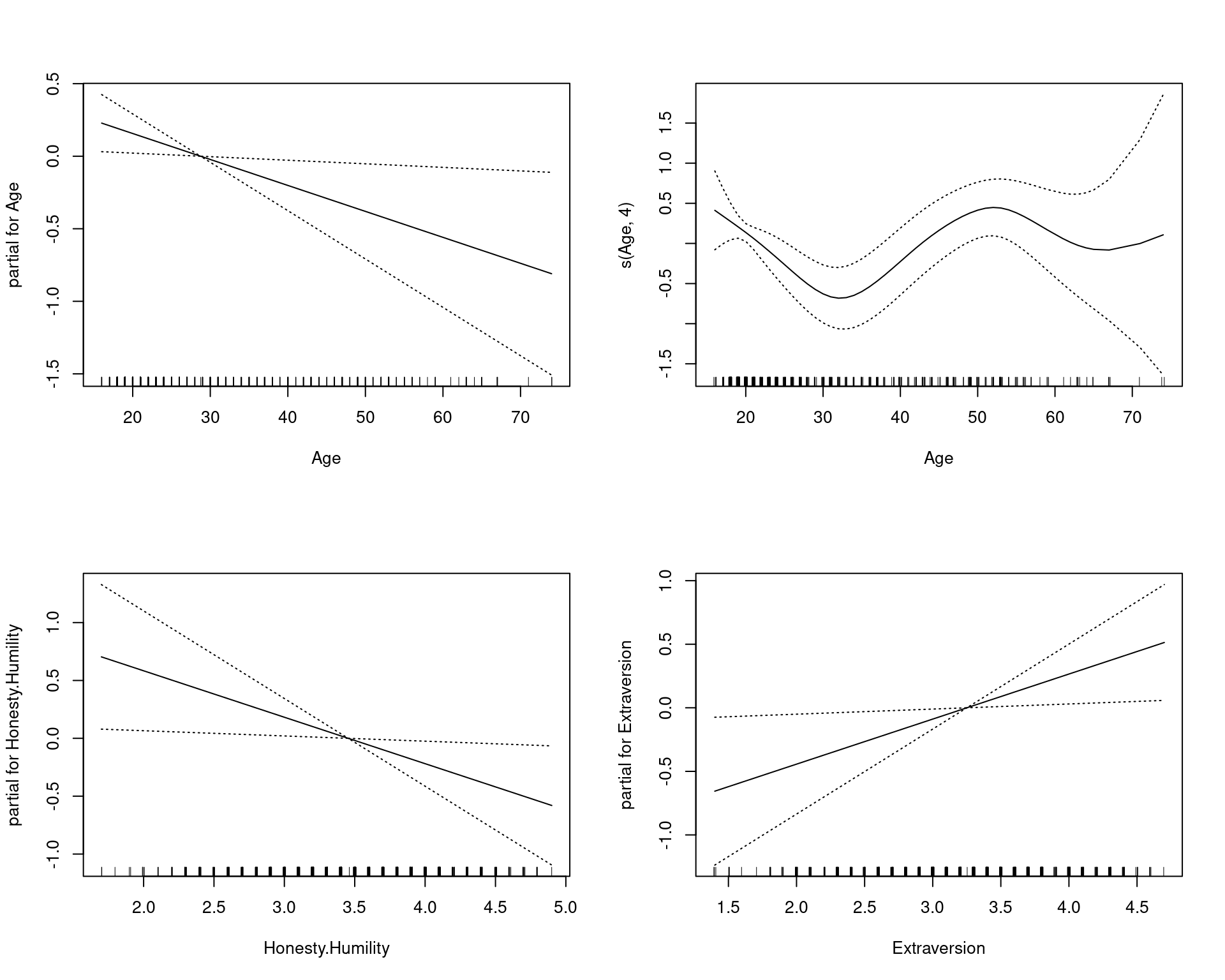
confusion(predict(step.model) > 0, iphone$Smartphone)Overall accuracy = 0.694
Confusion matrix
Predicted (cv)
Actual [,1] [,2]
[1,] 0.652 0.348
[2,] 0.284 0.716Notice the ANOVA separates out the parametric and non-parametric predictors because they need to be tested differently. Overall, the prediction accuracy doesn’t change much by including these higher-order transforms, but it tells us something about the relationship that may be informative. If we find non-linearities, it can reveal important things about the causal relationship that we would never see if we just assumed all relationships are linear.