
Knot insertion is a fundamental algorithm in curve and surface design. Its goal is to add one or more knots to the knot vector without changing the shape of the curve. Due to the fundamental identify m = n + p + 1, where m+1, n+1 and p are the number of knots, the number of control points, and the degree of a B-spline/NURBS curve, increasing the number of knots causes the number of control points to be increased the same amount. Thus, the existing set of control points must be modified to accommodate the increase of knots.
Although one can insert several knots at the same time, this system chooses to do it one-by-one for you to see and understand the effect of knot insertion. Follow the steps below to insert a knot:
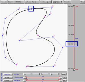
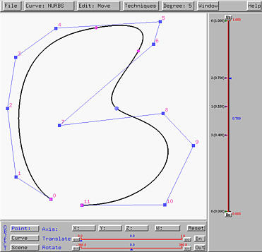
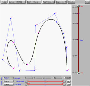
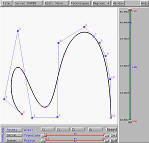
The following is a NURBS curve of degree 4 defined by 10 control points. We want to insert a new knot at u = 0.85. Since 0.85 is not an existing knot, the tracing point is not on any knot point.
Selecting Techniques followed by Knot Insertion yields the left figure below. As you can see, we have one more knot at u = 0.85 and the number of control points is increased by one. If we put the new and the original control polygons together, as shown in the right figure below where the new control points are marked with blue rectangles, you will see that the polyline defined by control points 5, 6, 7, 8 and 9 is modified by cutting the corners at 6, 7 and 8. In this way, one new control point is created.
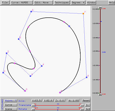
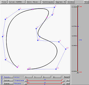
The following is a NURBS curve of degree 5 defined by 12 control points. This NURBS curve has knots 0 (multiplicity 6), 0.4 (multiplicity 3), 0.55 (simple), 0.7 (multiplicity 2) and 1 (multiplicity 6). We want to insert a new knot at 0.7, making knot 0.7 a triple knot after the insertion.
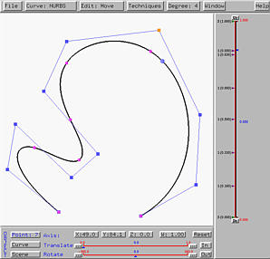
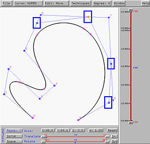
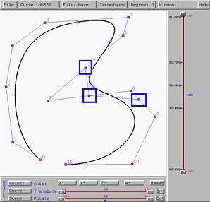
Move the u-indicator to 0.7 and select Techniques followed by Knot Insertion. This gives the left figure below. Now the curve is defined by 13 control points and those control points near the tracing point at u = 0.7 are modified. To see the modification, let us put the new and the original control polygons together as shown in the right figure below. You should see that the affected polyline is defined by the original control points 6, 7, 8 and 9, and that the corners at 7 and 8 are cut to create the three new control points marked by blue rectangles.
In general, if p is the degree of a B-spline/NURBS curve, s is the multiplicity of the new knot before insertion, and c is the number of corners to be cut, then we always have p = s + d.
How to overlay two curves and their control polygons You can save the first curve and then work on the second. Finally, import the first curve back on the canvas.

Knot insertion is a very useful algorithm that can be used in many applications, including an implementation of de Boor's algorithm. Here, we shall show you some important facts.
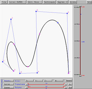
The left figure below is a NURBS curve of degree 4 defined by 8 control points. The figure also shows the tracing point corresponding to u = 0.9, which is not a knot. Click here to download a copy of this scene to file knot-insert.dat. If u = 0.9 is inserted as a new knot, three corners are cut and the result is shown in the right figure below.

If u = 0.9 is inserted again, it is inserted at an existing knot, making 0.9 a double knot. The result is shown in the left figure below. If 0.9 is inserted the third time, this will makes 0.9 a triple knot and the result in the right figure below suggests that line segment of control points 6 and 7 is tangent to the curve at the tracing point. In fact, if p is the degree and u is a knot of multiplicity p - 1, then the curve is tangent to a line segment of the control polygon at the point on curve corresponding to u.

If u = 0.9 is inserted the fourth time, the point on the curve corresponding to the knot becomes a control point (i.e., it has a control point index)! More precisely, if u is inserted so that the multiplicity after insertion is equal to the degree of the curve, then the point on the curve corresponding to u is a control point. That is, the curve passes through one of its control points. In face, de Boor's algorithm is implemented this way. Given a u, to find its corresponding point on the curve, we can repeatedly insert u until its multiplicity is equal to the degree of the curve. Then, the last control point is the desired point that corresponds to this u. This is shown in the figure below.
It is impossible to remove a knot without changing the shape of the curve. Therefore, this system implements "knot splitting" for splitting a multiple knot. However, the shape of the curve will change slightly.
You can move the u-indicator to a multiple knot. Then, select Techniques followed by Knot Splitting. The multiple knot will be split into two. If the multiple knot is of multiplicity k, after splitting the multiple knot will have multiplicity k - 1, and a new simple knot will be created nearby. Of course, the shape of the curve will change; however, if the newly created simple knot is moved to its "parent" multiple knot, the curve will return to its original shape.
The left figure below is a NURBS curves of degree 5 with knots 0 (multiplicity 6), 0.4 (multiplicity 3), 0.55 (simple knot), 0.7 (multiplicity 2) and 1 (multiplicity 6). This curve was used earlier on this page. Click here to download a copy of this file knot-split.dat. The u-indicator is at u = 0.4, the first internal knot. Its tracing point is also shown. Selecting Techniques followed by Knot Splitting yields the right figure below. The triple knot 0.4 is split into two, one double knot at 0.4 (the original place) and one simple knot 0.38. It is hard to see the difference between the following two curves. However, if you import the original file into the scene after the triple knot is split and use different colors for the curve segments, you should be able to see some very subtle difference between the two curves. Thus, unlike knot insertion, knot splitting does not preserve the shape of the curve.