A Quick Tour

This program uses the left mouse button exclusively

After launching the curve system you should see the following two windows:

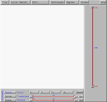
The left one is the drawing canvas on which you design your curve. The right one is the Display & Options Window, which contains various display options.

Exiting the Program

To exit this program, select File followed by Exit.

Creating Control Points

The drawing canvas is the xy-plane with the x-axis running from left to right and the y-axis running from bottom up. The coordinate origin is at the center of the drawing canvas.

The first step of designing a curve is putting some control points on the drawing canvas, the big square area. This requires the following steps:

Select Edit followed by Create. The pointer changes to a cross indicating that the program is in the insert mode.
Move the pointer to the drawing canvas and click at various locations. Each click creates a control point shown as a little square with a number attached, the control point number. Note that control point numbers start with 0.
After adding all control points, the curve system must be told about the curve type you want. Although this program supports Bézier, rational Bézier, B-spline and NURBS curves, Bézier curves will be used in this tour exclusively. By default, the curve type is Bézier. But you can always change this default by selecting Curve, followed by New Curve Segment, followed by the type of the curve (e.g., Bézier, rational Bézier, B-spline and NURBS), followed by Show Curve Segment. 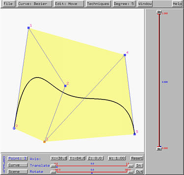The curve defined by the control points will be shown. In the following, six control points and the corresponding Bézier curve are shown.

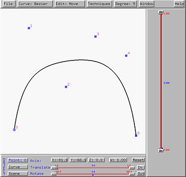
The degree of the Bézier curve is shown in the Degree button. Since there are six control points, the degree of this Bézier curve is 5.

Changing the Positions of Control Points

Changing the position of a control point is easy, even though a curve has already been displayed. To move a control point, the first thing to do is leaving the insert mode. To do so, choose Edit followed by Move. After this, the pointer is changed to a north-west pointing arrow indicating that the program is in move mode.

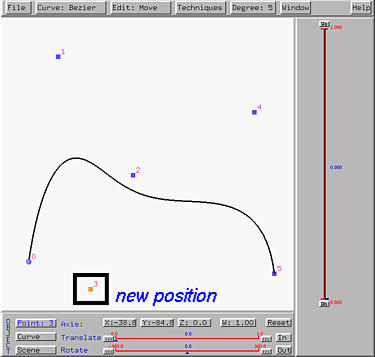
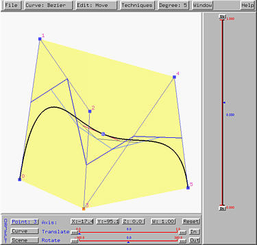
In move mode, one can move the pointer to a control point, drag it to a new location, and then release the mouse button. As the control point moves, the shape of the curve changes on-the-fly. Let us move control point 3 downward, the shape of the curve is pulled downward as shown below:

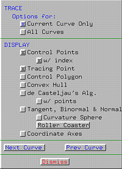
Control Polyline and Convex Hull

The Display & Options Window has a number of buttons and is subdivided into four parts. Selecting one of these button by clicking on it either activates or deactivates the corresponding option. If an option is active currently, the button shows a x. Clicking on an active (resp., inactive) button will deactivate (resp., activate) it.

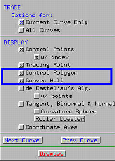
Activating Convex Hull displays the convex hull of the control points. Activating Control Polygon displays the control polyline. The following shows the control polyline and convex hull of the given control points:

Curve Tracing

To trace the curve use the vertical slider. The range of this slider is 0 and 1. The current position of u is marked by a small triangle, the u-indicator, and its value is shown in the middle of the slider. As the u-indicator moves along the slider up and down, its value is shown and a small dot, which indicates the point on the curve corresponding to the current value of u, moves on the curve. In the following figure, the u-indicator is moved to 0.45 (i.e., u = 0.45) and the corresponding point on the curve is near control point 2.

De Casteljau's Algorithm

If de Casteljau's alg. is activated, all intermediate polylines of the computation of de Casteljau's algorithm will be shown. As u moves, this net of polylines moves as well. The following shows a snapshot of this feature. Note that different polylines are shown in different colors.

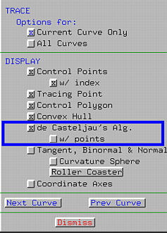
To make the polylines clearly shown, one might activate w/ point to show the vertices of polylines.

Partition of Unity

Since Bézier basis functions play an important role in generating the curve, this program can display these basis functions and partition of unity. To do so, choose Window followed by Partition of Unity. The Partition of Unity Window appears and shows all basis functions. To dispose this window, select the Dismiss button at the lower left corner of this window.

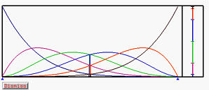
In our example, there are six control points and hence six basis functions, one for each control point. Each of these six basis functions are shown with a different color. As u moves by dragging the u-indicator with the vertical slider, its position will also be shown in this partition of unity window with a vertical bar. At the right end of this window, values of all basis functions at u are arranged into a vertical line segment showing the way of partitioning of unity. As u changes, the way of partitioning of unity changes as well. The above figure shows the way of partitioning of unity at u = 0.5.