


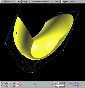
After launching the surface program you should see the following two windows:
The left one is the drawing canvas which is currently showing a default surface with a black background, while the right one is called the Tracing Window for you to control and trace the displayed surface.


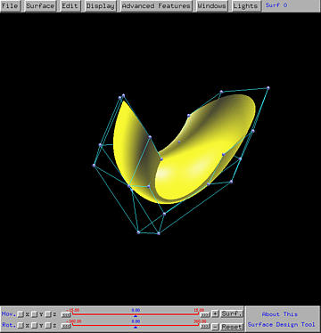
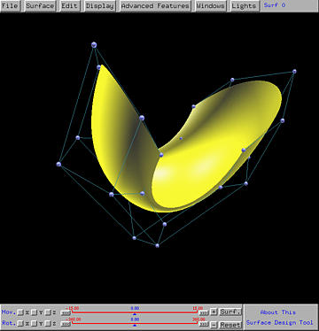
All control points are shown as little white spheres.
After perspective projection is activated, the menu option becomes Switch to Parallel Projection for you to switch back to parallel projection.
Note that all display options under Display will either show Show ... or Hide .... After an option is activated, the opposite will be shown in the menu.
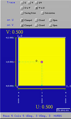
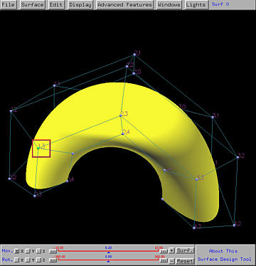
The big square in the middle is the unit square domain of the surface being displayed (i.e., [0,1]×[0,1]), where the u-direction is horizontal and the v-direction is vertical. Numbers below and to the left of the domain are knots. They are always in pairs with the first the multiplicity and the second the knot value.
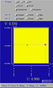
There is a circular dot, the uv-indicator, with two dashed line segments giving its u value and v value. This is a point (u,v) that can be dragged in the unit square. As this indicator moves, the corresponding u and v values, which are shown in yellow, also change. To see the corresponding point on the surface, click on the Tracing Point button on the top part of this window. Then, the corresponding points on the surface is shown as a red sphere. The following shows the tracing point on the surface corresponding to (0.9, 0.53):
To deactivate this display option, click on the Tracing Point button again.
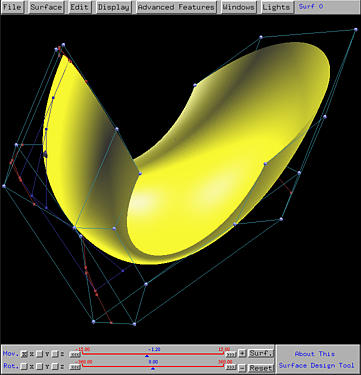
As the uv-indicator in the Tracing Window moves, the red sphere on the surface as well as all intermediate polylines move accordingly.
To deactivate this display option, click on the Calculation button again.
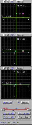
Dragging the little disk in the top window will cause the selected control point moving in the xy direction. More precisely, as the little disk moves, the x- and y-coordinate values of the selected control point will change and the z-coordinate is kept the same. Similarly, the second and the third windows are for moving a selected control point in the xz and yz directions, respectively. The x-, y- and z-coordinate and the weight w (if the surface is a NURBS surface) are displayed in the bottom of this window.
When the mouse pointer is in this window, clicking the right button pops up a menu with two items Large Steps and Small Steps. The former allows you to move the selected control point in a larger step size and the latter allows to use smaller step size.
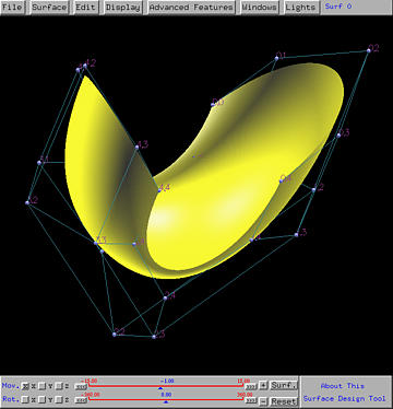
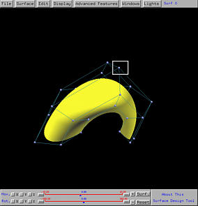
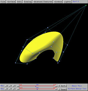
The following left figure shows a selected control point. After moving in the xy direction to a new position, the shape of the surface is changed (the right figure). In fact, part of the surface is pulled in the moving direction of the selected control point.
The Reset buttons on the top of each small window reset the control point back to the position before this move, and the Dismiss button closes this window. Note that resetting may not be very accurate due to the fact that some mouse activities may not be caught precisely.

To perform a translation or a rotation to the scene or to the surface, you must select the object to be transformed and a reference coordinate axis. For example, to translate the scene in the y-direction, one must click on the Surf. button to make Scene to appear. However, if Scene is shown, the transformation will be applied to the scene. Then, select Y and drag the Move slider. This will cause the whole scene moved in the y direction. You can also click on button >>> (resp., <<<) to increase (resp., decrease) the amount of translation and rotation.
To zoom in (i.e., moving the camera closer to the surface), use button +; and to zoom out (i.e., moving the camera farther way from the surface), use button -.
This system supports a second way of performing translations and rotations to the scene. Here is how.
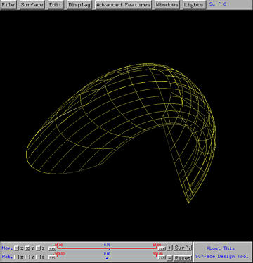
If your machine is not fast enough, some mouse movements would not be caught on time and some many even lost. As a result, the sliders may not be able to provide accurate movements. If this happens, use wireframe display method.
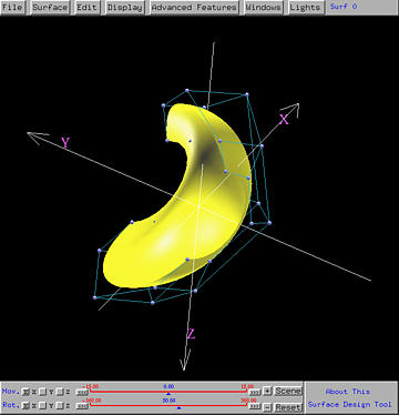
In many cases, having the coordinate axes shown will help to position the surface or the scene to a desired place. You can select Display followed by Show Axes to display the coordinate axes or Hide Axes to hide the coordinate axes.
To close this window, select the Dismiss button at the lower left corner of this window.
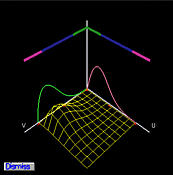
The above left figure shows a B-spline surface with control point 1,3 (i.e., row 1 and column 3) selected. Thus, the Partition of Unity window shows N1,p(u) in the u direction and N3,q(v) in the v direction. Note that p and q are the degrees in the u and v directions. The product, N1,p(u)N3,q(v), is the coefficient (i.e., two-dimensional basis function) for control point 1,3.
To use this polygonizer, click on Surface followed by Implicit Surface. This will load the polygonizer into this system. Before you can display a surface, an implicit equation must be given. If you choose Define Implicit Surface, your will see a window for you to type in your equation that defines the surface. In fact, you type in the equation through a text editor running in the newly opened window. You can also select Define Your Editor to choose your favorable editor. Note that this editor must be accessible via the current path.
What you have to do are (1) declaring variables you want to use in the function myfunc() and (2) returning the result of evaluating your implicit equation with variable rsq. For example, the torus in a "standard" position has the following implicit equation:
(x2 + y2 + z2 - ( R2 - r2))2 - 4R2(r2 - z2) = 0
Function myfunc() should be
double myfunc (double x, double y, double z)
{
    double rsq;  /* return value    */
    double R = 2.0, r = 1.0, temp;

    temp = x*x + y*y + z*z - (R*R + r*r);
    rsq  = temp*temp - 4.0*R*R*(r*r - z*z);
    return rsq;  /* must return this value */
}
Then, save your equation, wait for a while and the drawing canvas will
display a torus:
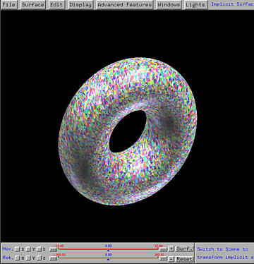
The polygonizer subdivides the surface of the torus into 31068 triangles with 15534 vertices. Each triangle is displayed with a random color as shown in the above figure.
When this implicit surface feature activated (i.e., an implicit surface is shown on the drawing canvas), You can only translate and rotate the scene, and you must use the sliders for translations and rotations, and + and - for zooming.
To switch back to parametric surfaces, select Surface, followed by Unload Implicit Surface.