The Centripetal Method

E. T. Y. Lee proposed this centripetal method. Suppose we are driving a car through a slalom course. We have to be very careful at sharp turns so that the normal acceleration (i.e., centripetal force) should not be too large. Otherwise, our car may lose control. To drive safely, Lee suggested that the normal force along the path should be proportional to the change in angle. The centripetal method is an approximation to this model. In fact, we can consider the centripetal method as an extension to the chord length method.

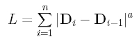
Suppose the data points are D₀, D₁, ..., D_n. First of all, we should select a positive "power" value a. Usually, it is a = 1/2 for square root. Then, the distance between two adjacent data points is measured by |D_k - D_k-1|^a rather than the conventional |D_k - D_k-1|. The length of the data polygon under this new measure is

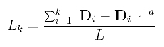
The ratio of the distance from D₀ to D_k on the data polygon over the total length is

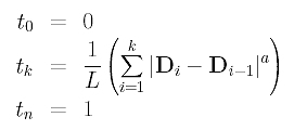
Therefore, L₀ = 0, L₁, ..., L_n = 1 divide [0,1] according to the length of data polygon under the new distance measure. Hence, the parameters are

If a = 1, the centripetal method reduces to the chord length method, and, hence, the former can be considered as an extension to the latter. If a < 1, say a = 1/2 (i.e., square root), |D_k - D_k-1|^a is less than |D_k - D_k-1|. Consequently, the impact of a longer chord (i.e., length > 1) on the length of the data polygon is reduced, and the impact of a shorter chord (i.e., length < 1) on the length of the data polygon is increased. Because of this characteristic, Lee claimed that the centripetal method handles sharp turns better than the chord length method.

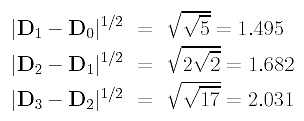
Let us redo the example discussed in the chord length method. We have four data points (n = 3): D₀ = < 0,0 >, D₁ = < 1,2 >, D₂ = < 3,4 > and D₃ = < 4,0 >. Choose a = 1/2 and the length of each chord under this new measure is

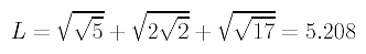
The total length is

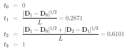
Therefore, the parameters are

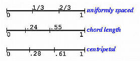
The following gives the distributions of three sets of parameters computed using the uniformly spaced method, the chord length method, and the centripetal method.

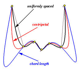
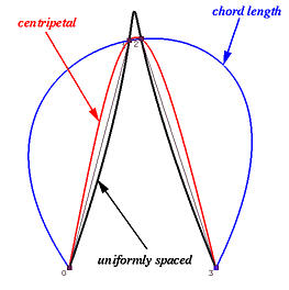
Let us take a look at an extreme example. The following shows four data points interpolated by three B-spline curves using the uniformly spaced method (in black), chord length method (in blue) and centripetal method (in red). As you can see, the uniformly spaced method has a peak, the chord length method have two big bulges, and the centripetal method interpolates the two very close adjacent points nicely.

Can we say the centripetal method is superior to the other two? The following example tells a different story. We have 7 data points and the black, blue and red curves are generated using the uniformly spaced method, chord length method and centripetal method. Now, the uniformly spaced method provides a very tight interpolation. The centripetal method is slightly off the the tight result using the uniformly spaced method. Finally, the chord length method wiggles through the two longest chords too much!