Surface Global Interpolation

Suppose we have m+1 rows and n+1 columns of data points D_ij (0 <= i <= m and 0 <= j <= n) and wish to find a B-spline surface of degree (p,q) that contains all of them. Similar to the curve case, we have data points and degrees p and q as input. To define an interpolating a B-spline surface, we need two knot vectors U and V, one for each direction, and a set of control points. Like the curve case, the number of control points and the number of data points are equal (i.e., (m+1)×(n+1) control points in m+1 rows and n+1 columns). With the technique discussed in Parameters and Knot Vectors for Surfaces, we can compute two sets of parameters s_c (0 <= c <= m) in the u-direction and t_d (0 <= d <= n) in the v-direction by setting e and f to m and n, respectively. We also obtain knot vectors U and V for the u- and v-direction, respectively. Therefore, what remains is to find the desired control points!

Finding a Solution

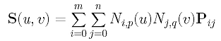
Suppose the B-spline surface is given as follows:

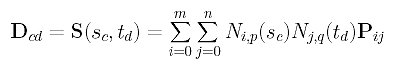
Since it contains all data points and since parameters s_c and t_d correspond to data point D_cd, plugging u=s_c and v=t_d into the surface equation yields:

Since N_i,p(s_c) is independent of the index j, it can be moved out of the summation of j:

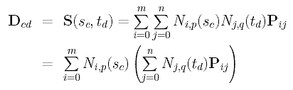
If we examine the inner term, we shall see that the index i only appears in P_ij. Therefore, we can define the inner expression to be a new term as follows:

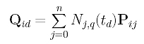
More precisely, if i is fixed to the same value, Q_id is the point, evaluated at t_d, on the B-spline curve of degree q defined by n+1 "unknown" control points on row i of the P's (i.e., P_i0, P_i1, ..., P_in). Plugging Q_id into the equation of D_cd above yields

Thus, data point D_cd is the point, evaluated at s_c, of a B-spline curve of degree p defined by m+1 "unknown" control points on column d of the Q's (i.e., Q_0d, Q_1d, ..., Q_md). Repeating this for every c (0 <= c <= m), the d-th column of data points (i.e., D_0d, D_1d, ..., D_md) is obtained from the d-th column of Q's (i.e., Q_0d, Q_1d, ..., Q_md) and parameters s₀, s₁, ..., s_m. Since data points D_0d, D_1d, ..., D_md, degree p and parameters s₀, s₁, ..., s_m are known, this equation means

So, it is a curve interpolation problem! More precisely, the curve global interpolation can be applied to each column of the data points to obtain a column of control points Q_cd's. Since we have n+1 columns of data points, we shall obtain n+1 columns of Q's.

Now, we can use the same idea but apply to the equation of Q_id, which is duplicated below. In this equation, data points on row i of the Q's (i.e., Q_i0, Q_i1, ..., Q_in) are the points on a B-spline curve, evaluated at t₀, t₁, ..., t_n, of degree q defined by n+1 unknown control points P_i0, P_i1, ..., P_in. Therefore, applying curve interpolation with degree q and parameters t₀, t₁, ..., t_n to row i of the Q's gives row i of the desired control points!

Once all rows of control points are found, these control points, along with the two knot vectors and degrees p and q define an interpolating B-spline surface of degree (p,q) of the given data points. Therefore, surface interpolation using B-spline consists of (m+1) + (n+1) curve interpolations! The following summarizes the required steps:

Note that matrix N used in the first for loop does not change when going from column to column. Therefore, if we naively follow the above algorithm, we would end up solving the system of equation D = N^.Q n+1 times. This is, of course, not efficient. To speed up, the LU-decomposition of N should be computed before the first for loop starts, and the interpolation in each iteration is simply a forward substitution followed by a backward substitution. Similarly, a new matrix N will be used for the second for loop. Its LU-decomposition should also be computed before the second for starts. Without doing so, we will perform (m+1)+(n+1)=m+n+2 LU-decompositions when only 2 would be sufficient.

Why Is This Method Global?

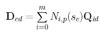
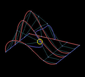
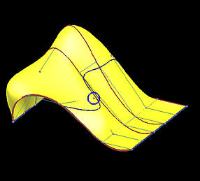
Because the interpolating surface is obtained through m+n+2 global curve interpolations, it is obvious that this interpolation technique is global. The following images show the impact of moving a data point. This B-spline surface is obtained by using six rows (m=5) and five columns (n=4) data points with degree (3,3). Images on the top row show the knot curves (i.e., isoparametric curves that correspond to knots), and the data point marked by a yellow circle indicates the point to be moved. The bottom row shows the corresponding rendered surfaces. It is obvious that after changing the position of a data point, the blue knot curve changes its shape drastically, and moves closer to its neighboring data points. The impact propagates to the right as well because the valley in the far right end is a little deeper as can be seen from the red knot curves. The more dramatic change is shown in the rendered surfaces. Although the indicated data point is moved to the right, this move creates a big bulge in the left end. Please also note that the front boundary curve, actually a red knot curve, also changes its shape slightly. Therefore, the impact of changing the position of a single data point can propagate to entire surface, and, hence, this is a global method.

	Before Move	After Move
Knot Curves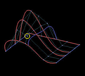
Surfaces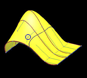