
In an algorithms design course, you learned complexity measures of algorithms. For example, an optimal sorting algorithm takes O(nlog(n)) comparisons, where n is the number of data items to be sorted. Although normally we do not count the number of steps for solving a geometric problem because it is not always possible (e.g., how many step are required to solve a non-linear equation using Newton's method?), understanding the complexity of a geometric problem would be very helpful.
Adrian Bowyer and John Woodwark distinguish three types of complexity in a geometric problem: namely, dimensional complexity, analytic complexity and combinatorial complexity.
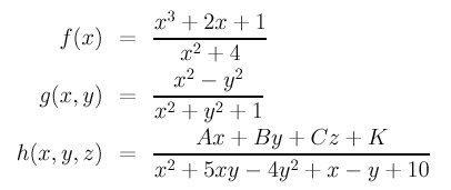
Beyond polynomials and rational polynomials, we have transcendental functions such as sin(), cos(), tan(), asin(), asin(), atan(), log() and exp(). All of these functions add extra complexity into the solution of a geometric problem.
Worse, in many cases an equation does not tell us the actual geometric intent at all. For example, x2 - y2 -2y -1 = 0 is a quadratic equation because the highest degree is 2. But, it is not a conic curve (i.e., an ellipse, hyperbola or parabola); it actually represents two lines, x + y + 1 = 0 and x - y - 1 = 0, because it can be factorized as (x + y + 1)(x - y - 1) = 0. An equation may not represent any point (well, any REAL point) in a plane. For example, what is the graph of x2 + y2 + 1 = 0? Since the square of any real number must be positive, the left-hand side (i.e., x2+y2+1) is always positive and hence there exists no real points that can satisfy this equation.
In some geometric operations such as intersection computation the situation can become very nasty. Detecting if a line and a surface intersect is a common operation in raytracing. However, this is definitely not an easy job, and if the surface is a complex one this job could become much more difficult. Why? In three-dimension, a line can be written as
where t is a parameter. Plugging (x,y,z) into the equation of a surface, say f(x,y,z)=0, yields f(a+tu,b+tv,c+tw)=0. Rearranging gives us a polynomial in t:

Solving for t gives the intersection points. Mathematically it is done. Since it is well-known (in mathematics) that polynomials with degree higher than four do not have closed-form solutions. That means, numerical methods is required to solve the above equation. We have two problems here:
If polynomials are the major tools for solving geometric problems, the number of coefficients of a polynomial, which depends on the degree of the polynomial and the number of dimensions, adds another level of complexity. For an example, a polynomial of two variables, which described a curve in the xy-plane, has (n+1)(n+2)/2 coefficients. More precisely, a line is a degree 1 polynomial and has three coefficients (e.g., Ax+By+C=0); a conic curve is a degree two curve and has six coefficients (e.g., Ax2+Bxy+Cy2+Ex+Ey+F=0); and a cubic curve is a degree three polynomial and has 10 coefficients (e.g., Ax3+Bx2y+Cxy2 +Dy3+Ex2+Fxy+Gy2+Hx+Iy+J=0). Therefore, the number of coefficients (or terms) of degree n polynomial increases proportional to the square of n.
For polynomials of three variables, which describe surfaces in space, the number of coefficients (or terms) is (n+1)(n+2)(n+3)/6, where n is the degree of the polynomial. For example, a plane is a degree 1 polynomial and has four coefficients (e.g., Ax+By+Cz+D=0); and a quadric surface is a degree two polynomial and has ten coefficients (e.g., Ax2+By2+Cz2+Dxy+Exz+Fyz+Gx+Hy+Iz+J=0). Thus, the number of coefficients of a degree n polynomial increases proportional to the cubic of n. Based on this counting, a degree 3, 4 and 5 polynomial has 20, 35 and 56 coefficients. This rate of increase forces us to only use lower degree polynomials.
However, geometric problem could have yet another combinatorial complexity which is usually due to the number of different cases. For example, when developing a curve/surface system, one needs some functions for computing the intersection of the following cases: line and line, line and circle, circle and circle. If ellipses are supported by the system, one must consider the cases of line/ellipse, circle/ellipse and ellipse/ellipse. In general, if a system supports k different types of curves, one may need k(k-1)/2 functions, one for each possible combination. The story does not end here, because a system may have other type of objects (polyhedra and surfaces). Ok, you might want to say: let us develop a general algorithm that can compute the intersection points of any two types of curves. It is certainly doable and actually there have been many papers on this subject. The problem is that general algorithms usually are not reliable enough when used to solve special cases, cases that occur frequently in practice.