
Following the construction of a Bézier curve, the next important task is to find the point C(u) on the curve for a particular u. A simple way is to plug u into every basis function, compute the product of each basis function and its corresponding control point, and finally add them together. While this works fine, it is not numerically stable (i.e., could introduce numerical errors during the course of evaluating the Bernstein polynomials).
In what follows, we shall only write down the control point numbers. That is, the control points are 00 for P0, 01 for P1, ..., 0i for Pi, ..., 0n for Pn. The 0s in these numbers indicate the initial or the 0-th iteration. Later on, it will be replaced with 1, 2, 3 and so on.
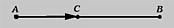
The fundamental concept of de Casteljau's algorithm is to choose a point C in line segment AB such that C divides the line segment AB in a ratio of u:1-u (i.e., the ratio of the distance between A and C and the distance between A and B is u). Let us find a way to determine the point C.
The vector from A to B is B - A. Since u is a ratio in the range of 0 and 1, point C is located at u(B - A). Taking the position of A into consideration, point C is A + u(B - A) = (1 - u)A + uB. Therefore, given a u, (1 - u)A + uB is the point C between A and B that divides AB in a ratio of u:1-u.
The idea of de Casteljau's algorithm goes as follows. Suppose we want to find C(u), where u is in [0,1]. Starting with the first polyline, 00-01-02-03...-0n, use the above formula to find a point 1i on the leg (i.e. line segment) from 0i to 0(i+1) that divides the line segment 0i and 0(i+1) in a ratio of u:1-u. In this way, we will obtain n points 10, 11, 12, ...., 1(n-1). They define a new polyline of n - 1 legs.
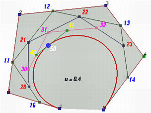
In the figure above, u is 0.4. 10 is in the leg of 00 and 01, 11 is in the leg of 01 and 02, ..., and 14 is in the leg of 04 and 05. All of these new points are in blue.
The new points are numbered as 1i's. Apply the procedure to this new polyline and we shall get a second polyline of n - 1 points 20, 21, ..., 2(n-2) and n - 2 legs. Starting with this polyline, we can construct a third one of n - 2 points 30, 31, ..., 3(n-3) and n - 3 legs. Repeating this process n times yields a single point n0. De Casteljau proved that this is the point C(u) on the curve that corresponds to u.
Let us continue with the above figure. Let 20 be the point in the leg of 10 and 11 that divides the line segment 10 and 11 in a ratio of u:1-u. Similarly, choose 21 on the leg of 11 and 12, 22 on the leg of 12 and 13, and 23 on the leg of 13 and 14. This gives a third polyline defined by 20, 21, 22 and 23. This third polyline has 4 points and 3 legs. Keep doing this and we shall obtain a new polyline of three points 30, 31 and 32. From this fourth polyline, we have the fifth one of two points 40 and 41. Do it once more, and we have 50, the point C(0.4) on the curve.
This is the geometric interpretation of de Casteljau's algorithm, one of the most elegant result in curve design.

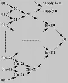
First, all given control points are arranged into a column, which is the left-most one in the figure. For each pair of adjacent control points, draw a south-east bound arrow and a north-east bound arrow, and write down a new point at the intersection of the two adjacent arrows. For example, if the two adjacent points are ij and i(j+1), the new point is (i+1)j. The south-east (resp., north-east) bound arrow means multiplying 1 - u (resp., u) to the point at its tail, ij (resp., i(j+1)), and the new point is the sum.
Thus, from the initial column, column 0, we compute column 1; from column 1 we obtain column 2 and so on. Eventually, after n applications we shall arrive at a single point n0 and this is the point on the curve. The following algorithm summarizes what we have discussed. It takes an array P of n+1 points and a u in the range of 0 and 1, and returns a point on the Bézier curve C(u).
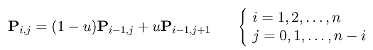
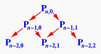
More precisely, entry Pi,j is the sum of (1-u)Pi-1,j (upper-left corner) and uPi-1,j+1 (lower-left corner). The final result (i.e., the point on the curve) is Pn,0. Based on this idea, one may immediately come up with the following recursive procedure:
This procedure looks simple and short; however, it is extremely inefficient. Here is why. We start with a call to deCasteljau(n,0) for computing Pn,0. The else part splits this call into two more calls, deCasteljau(n-1,0) for computing Pn-1,0 and deCasteljau(n-1,1) for computing Pn-1,1.
Consider the call to deCasteljau(n-1,0). It splits into two more calls, deCasteljau(n-2,0) for computing Pn-2,0 and deCasteljau(n-2,1) for computing Pn-2,1. The call to deCasteljau(n-1,1) splits into two calls, deCasteljau(n-2,1) for computing Pn-2,1 and deCasteljau(n-2,2) for computing Pn-2,2. Thus, deCasteljau(n-2,1) is called twice. If we keep expanding these function calls, we should discover that almost all function calls for computing Pi,j are repeated, not once but many times. How bad is this? In fact, the above computation scheme is identical to the following way of computing the n-th Fibonacci number:
The triangular computation scheme of de Casteljau's algorithm offers an interesting observation. Take a look at the following computation on a Bézier curve of degree 7 defined by 8 control points 00, 01, ..., 07. Let us consider a set of consecutive points on the same column as the control points of a Bézier curve. Then, given a u in [0,1], how do we compute the corresponding point on this Bézier curve? If de Casteljau's algorithm is applied to these control points, the point on the curve is the opposite vertex of the equilateral's base formed by the selected points!
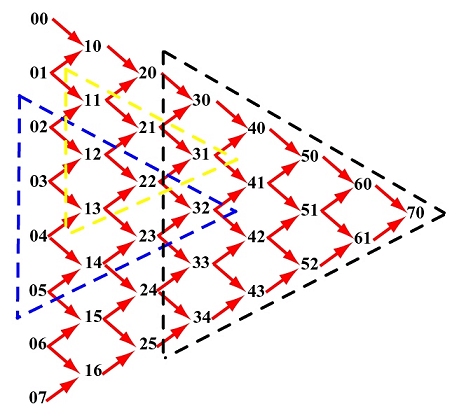
For example, if the selected points are 02, 03, 04 and 05, the point on the curve defined by these four control points that corresponds to u is 32. See the blue triangle. If the selected points are 11, 12 and 13, the point on the curve is 31. See the yellow triangle. If the selected points are 30, 31, 32, 33 and 34, the point on the curve is 70.
By the same reason, 70 is the point on the Bézier curve defined by control points 60 and 61. It is also the point on the curve defined by 50, 51 and 52, and on the curve defined by 40, 41, 42 and 43. In general, if we select a point and draw an equilateral as shown above, the base of this equilateral consists of the control points from which the selected point is computed.