NURBS: Definition

Let us consider the way of introducing homogeneous coordinates to a B-spline curve and derive the NURBS definition.

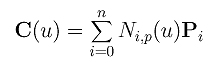
Given n+1 control points P₀, P₁, ..., P_n and knot vector U = { u₀, u₁, ..., u_m } of m+1 knots, the B-spline curve of degree p defined by these parameters is the following:

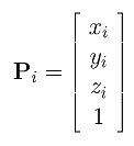
Let control point P_i be rewritten as a column vector with four components with the fourth one being 1:

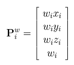
We can treat this P_i as a homogeneous coordinate. Since multiplying the coordinates of a point (in homogeneous form) with a non-zero number does not change its position, let us multiply the coordinates of P_i with a weight w_i to obtain a new form in homogeneous coordinates:

Note that P^w_i and P_i represent the same point in homogeneous coordinate. Plugging this new homogeneous form into the equation of the above B-spline curve, we obtain the following:

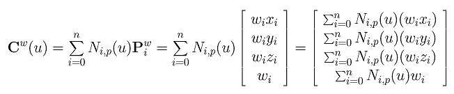
Therefore, point C^w(u) is the original B-spline curve in homogeneous coordinate form. Now, let us convert it back to Cartesian coordinate by dividing C^w(u) with the fourth coordinate:

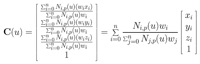
Finally, we have a clean form as follows:

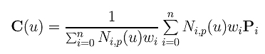
This is the NURBS curve of degree p defined by control points P₀, P₁, ..., P_n, knot vector U = { u₀, u₁, ..., u_m }, and weights w₀, w₁, .., w_n. Note that since weight w_i is associated with control point P_i as its fourth component, the number of weights and the number of control points must agree.

In general, weight w_i is positive; but negative weights have interesting applications. If a weight, say w_i, becomes zero, the coefficient of P_i is zero and, consequently, control point P_i has no impact on the computation of C(u) for any u (i.e., P_i is "disabled"). Moreover, zero weights also have a very useful interpretations called infinite control points.

Two Immediate Results

Here are two results available immediately from the above definition.

If all weights are equal to 1, a NURBS curve reduces to a B-spline curve.
This is obvious because in this case control points in homogeneous form are identical to their conventional Cartesian form and the denominator is 1.
NURBS Curves are Rational
This is also obvious. The value multiplied to control point P_i, N_i,p(u)w_i, is a polynomial of degree p. The denominator is the sum of all coefficients and hence is also a polynomial of degree p. As a result, the coefficient of control point P_i is the quotient of two degree p polynomials and function C(u) is rational.

These two results suggest that B-spline curves are special cases of NURBS curves. Moreover, since NURBS curves are rational, circles, ellipses and many other curves which are impossible with B-spline curves are now possible with NURBS curves.

A Geometric Interpretation

Are NURBS curves special kinds of curves? It turns out that they are not. In fact, they are simply another face of B-spline curves. Consider control points P^w_i = ( w_ix_i, w_iy_i, w_iz_i, w_i ). This point has four components and can be considered as a point in the four-dimensional space, and, consequently, C(u) below becomes a B-spline curve in the four-dimensional space:

In the discussion of a geometric interpretation of homogeneous coordinates, dividing the the first three coordinate components by the fourth one is equivalent to projecting a four-dimensional point to the plane w = 1. Since the above curve is converted to a NURBS curve by dividing the first three coordinates with the fourth, we conclude that a NURBS curve in the three-dimensional space is merely the projection of a B-spline curve in four-dimensional space. Therefore, if we know B-spline curves well, we should be able to know NURBS curves easily.