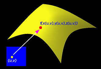

There are two types of surfaces that are commonly used in modeling systems, parametric and implicit. Parametric surfaces are defined by a set of three functions, one for each coordinate, as follows:
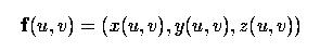
f(u,v) = ( x(u,v), y(u,v), z(u,v) )where parameters u and v are in certain domain. For our purpose, we shall assume both u and v are in the range of 0 and 1. Thus, (u,v) is a point in the square defined by (0,0), (1,0), (0,1) and (1,1) in the uv-coordinate plane. The following figure illustrates this concept.
Implicit surfaces, on the other hand, are defined by a polynomial of three variables:
p(x,y,z) = 0Similar to curves, if x(u,v), y(u,v) and z(u,v) are polynomials, parametric surfaces will not be able to represent many surfaces that are normally described by implicit surfaces. The sphere is a good example. You can easily prove this fact with an argument similar to that used for circles. If x(u,v), y(u,v) and z(u,v) are rational polynomials (i.e., quotients of two polynomials), parametric surfaces can represent spheres, ellipsoids and many other surfaces. However, similar to curves, many implicit surfaces do not have any parametric form. Therefore, in terms of expressive power, implicit surfaces are more powerful than parametric surfaces.
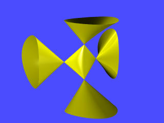
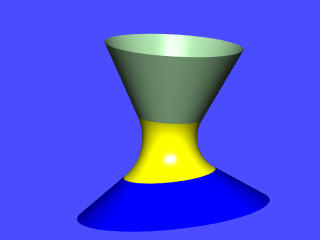
Here are a few technical terms. Surfaces which have polynomial (implicit) forms are called algebraic surfaces. The highest degree of all terms is the degree of the algebraic surface. Therefore, spheres and all quadric surfaces are algebraic surfaces of degree two, while torus is a degree four algebraic surface. The following shows a degree 3 algebraic surface whose implicit equation is
8x2 - xy2 + xz2 + y2 + z2 - 8 = 0
Some algebraic surfaces have rational parametric forms such as spheres and all quadric surfaces. This type of algebraic surfaces are called rational algebraic surfaces. Theoretically, given an algebraic surface in rational parametric form, it is always possible to eliminate parameters u and v so that the result is in an implicit form. This process (from parametric to implicit) is called implicitization. However, not all algebraic surfaces are rational. Unfortunately, determining if an algebraic surface is rational is very difficult, although algebraic geometry has provided such characterization theorems. Computationally, it is infeasible.

To compute the tangent and normal vector at a point (u,v) in the domain, we need the partial derivatives. Suppose the parametric surface is defined as follows:
The partial derivatives with respect to u and v are the tangent vectors at f(u,v):
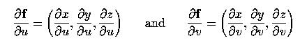
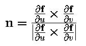
In the above, the left one is the tangent vector in the u-direction while the right one is the tangent vector in the v-direction. The normal vector at f(u,v), n(u,v), is the cross-product of these partial derivatives using the right-handed rule:
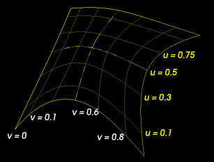
A parametric surface patch can be considered as a union of (infinite number) of curves. There are many ways to form these unions of curves; but, the simplest one is the so-called isoparametric curves. Given a parametric surface f(u,v), if u is fixed to a value, say 0.1, and let v vary, this generates a curve on the surface whose u coordinate is a constant. This is the isoparametric curve in the v direction with u = 0.1. Similarly, fixing v to a value and letting u vary, we obtain an isoparametric curve whose v direction is a constant. Therefore, let u be fixed at 0, 0.1, 0.1, ..., 0.9 and 1, we shall have 11 isoparametric curves f(0,v), f(0.1,v), f(0.2,v), ..., f(0.9,v) and f(1,v). These curves sweep out the surface if we let u change from 0 to 1 continuously. Similarly, the isoparametric curves generated by varying v cover the surface. The following figure shows a few isoparametric curves in both directions.
These isoparametric curves can help to render the surface. In many applications, a parametric surface is "triangulated" (or polygonized or tessellated) into triangles or polygons. Then, these triangles and polygons can be rendered very efficiently with existing graphics programming libraries such as OpenGL and PHIGS PLUS.
Instead of triangulating the surface, it would be easier to triangulate the domain of (u,v). We can subdivide the u-direction into m segments with u0=0, u1, ..., ui, ..., um=1 and subdivide the v-direction into n segments with v0=0, v1, ..., vj, ..., un=1. The domain is subdivided into m×n rectangles, each of which can be further subdivided into two triangles.
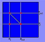
Suppose ui and ui+1 are two consecutive division points in the u-direction and vj and vj+1 in the v-direction as shown above. We have a rectangle in the domain with vertices (ui,vj), (ui+1,vj), (ui+1,vj+1) and (ui,vj+1). We have two ways to obtain the triangles because this rectangle has two diagonals. Let us follow the figure shown above. The first triangle is defined by (ui,vj), (ui+1,vj) and (ui,vj+1) and the second triangle is defined by (ui+1,vj), (ui+1,vj+1) and (ui,vj+1).
Consider the triangle defined by (ui,vj), (ui+1,vj) and (ui,vj+1). These three points are mapped to three points on the surface f(ui,vj), f(ui+1,vj) and f(ui,vj+1) with normal vectors n(ui,vj), n(ui+1,vj) and n(ui,vj+1). Now, we have three vertices each of which has a normal vector. These six pieces of information are sufficient to render the triangle smoothly. As a result, we have a method for rendering a parametric surface. Or, put it in another way, we have a method for generating a set of triangles that approximate the given parametric surface. This approximation may not be a good one because it could have too many triangles and some of these triangles may be in wrong positions or too small. This situation, however, can be improved by an "adaptive" technique. An adaptive technique dynamically adjusts the sizes, the number and the positions of triangles.
In addition to blending, many applications and computations such as offsetting naturally generate algebraic surfaces. In fact, in many cases, algebraic surfaces are very useful. Point classification is a good example. Point classification determines if a given point lies inside, on or outside of a surface. It is not easy to design an algorithm for parametric surface; however, for implicit surfaces it is a simple matter. Suppose the given point is (a,b,c) and the implicit surface is given by p(x,y,z)=0. Then, if p(a,b,c) is greater than, equal to or less than zero, (a,b,c) lies outside, on or inside of the surface.
One can easily compute the normal vector of an algebraic surface. In fact, the formal vector of a polynomial p(x,y,z) = 0 is simply its gradient:
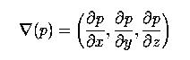
Once we have the normal vector at a point, the tangent plane can be easily computed.
Unfortunately, displaying an algebraic surface is not easy. The easiest but also the most time consuming way is raytracing. Many raytracers allow users to specify an implicit equation. POVRAY and Radiance are good examples. However, raytracing is very slow. Another possibility is triangulating the surface which is similar to what we did earlier for parametric surfaces. For implicit surfaces, however, situation is different because we do not have a domain to triangulate. More precisely, triangulation must be carried out directly on the surface. Programs that can subdivide an implicit surface into polygons (not necessarily triangles) are usually referred to as polygonizers. Developing such polygonizers is not an easy job and is still a research problem.
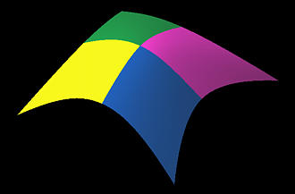
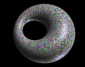
The following surfaces are generated from a well-known polygonizer by Jules Bloomenthal which has been incorporated into our surface system. The left surface is a hyperbolic paraboloid and the right one is a ring Dupin cyclide which is a degree 4 rational surface. These two surfaces are triangulated into a large number of small triangles each of which is colored with a random color. However, it is not necessary to have such a large number of triangles.
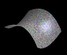
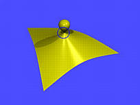
The first is a cubic surface whose equation is
x2 + y3 - y2 + z2 = 0The gradient of this surface is
( 2x, 3y2 - 2y, 2z )Therefore, (0,0,0) is a singular point because at this point all components of the gradient are zero. This is the indicated point on the surface. Note that there is another singular point at (0,2/3,0).
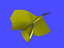
The middle figure has an equation as follows:
-x3 + 2xz - yz2 = 0This surface has the following gradient vector
( -2x2 + 2z, -2yz, 2x - y2 )From the second component, we have either y = 0 or z = 0. If y = 0, the third component forces x to be zero and hence the first component forces z to be zero. If z = 0, the first component forces x to be zero and the third component forces x to be zero. Both causes yield the singular point (0,0,0).
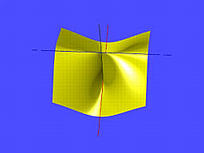
While the first two cases have only isolated singular points, singular points can be on a line or even on a curve. Let us consider the right figure above which has the following equation:
-x2y + x2 - yz2 - z2 = 0This surface has the following gradient vector
( -2xy+2x, -(x2+z2), -2z )If z = 0, the second component implies that x must also be zero. If both x and z are zero, the first component will also be zero no matter what values y may have. This means that as long as x = z = 0 and y has an arbitrary value we have a singular point. Therefore, the y-axis contains all singular points. The figure shows three lines. All of them lie on the surface; however, the vertical line is the y-axis which is also the self-intersection line containing all singular points.