(For the following problems, you will need the differential equation solver.  Please click here to access a short tutorial on how to use ode45.)

1. Wei-Prater Kinetics.

Using the data given in the following links:
    www.chem.mtu.edu/~tbco/cm5100/wpdata1.dat
    www.chem.mtu.edu/~tbco/cm5100/wpdata2.dat
    www.chem.mtu.edu/~tbco/cm5100/wpdata3.dat
    www.chem.mtu.edu/~tbco/cm5100/wpdata4.dat
(You can also download the m-functions I wrote that could help you plot the ternary diagrams:
draw_ternary.m
plot_ternary.m
getPoints_ternary.m
plus the short tutorial on what these commands do. )

Determine the rate constants for the process shown in Figure 1 where the reactions are all first order kinetics.



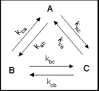
Figure 1. Three Simultaneous Reversible Reactions for Wei-Prater Data.

Suppose you have the for the differential equation: dx/dt = Ax, where the matrix A is given by,

>> A=1e4*[-1.0002, 0.0002, -0.9998;

-1.0003, 0.0003,-0.9997;
0.0002, -0.0002, -0.0002];
• Try using ode45 as before, simulating from 0 to 100. What happens ?
• Now try using ode15s instead. What happens ? Plot the results
• Check the eigenvalues of A and discuss the range of eigenvalues.

 
Note: Varying the order of magnitudes in eigenvalues is just one instance where equations are "stiff", there are known cases where the eigenvalues are not far apart and yet the normal RK methods do not perform well. There are other methods also available in Matlab to solve stiff problems (you can use the help files to learn more.)

For linear boundary value problems given by



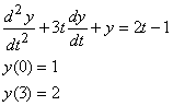
Method 1: using superposition.

Let v be the solution obtained using solvers such as ode45 with initial conditions, v(0)=1 (which is y(0)), and  dy/dt(0)=any.

>> [t1,v] = ode45(@diffeqn, [0:0.1:3], [1 ;1]);

Notes:

• You need to supply/create the m-file for the differential equations such as diffeqn.m that describes your system
• Explicitly state the intervals in the range of your independent values: [0:0.1:3]
• For v, we are using the same initial value, y(0) but choosing the dv/dt(0) =1.

• We use the same explicitly stated the intervals in the range of independent values: [0:0.1:3]
• For w, we are using the null initial value, w(0)=0 but choosing the dw/dt(0) =1.

Plot y as a function of t and see if it satisfies the boundary conditions.
( There are several other methods for solving boundary value problems, ranging from shooting methods to finite element methods. Matlab has the command  bvp4c  to handle not only linear, but several nonlinear, boundary value problems. See help files to explore these functions.)

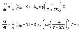
The following equations describe the dynamics equations of a CSTR:



Suppose the parameters of the process are given by the following values:

t	120
Cin	0.9
a	2000
ko	0.1
b	-1550
q	0.2
Tin	40

a) Obtain the equilibrium points of the given process. (Hint: first set dC/dt=f(C,T)=0
    to find C in terms of T, i.e. C=h(T). then substitute this function into dT/dt=0=f(C,T)
    to solve for T.)
b) At each of the equilibrium points, predict the behavior of the phase space
    in the neighborhood of these points, i.e. will it be a stable node, unstable
    node, saddle, unstable focus or stable focus.
c) Simulate the process at various initial conditions. For instance,
    using matlab, you could use the following commands:
 

for i = 0.6:0.1:1
    [t,x]=ode45(@cstr,[0 1000],[i 20]);
    plot(x(:,1),x(:,2));
    hold on
end

for i = 20:10:200
    [t,x]=ode45(@cstr,[0 1000],[0.6 i]);
    plot(x(:,1),x(:,2));
    hold on
end

for i = 20:10:200
    [t,x]=ode45(@cstr,[0 1000],[1 i]);
    plot(x(:,1),x(:,2));
    hold on
end
axis([0.6 1 0 400])
 

where the model for the process is given in the file cstr.m given by:   function dx=cstr(t,x)
    ko=0.1;
    tau=120;
    Cin=0.9;
    alpha=2000;
    beta=-1550;
    q=0.2;
    Tin=40;
    C=x(1);
    T=x(2);
    rate = ko*exp(-alpha/(T+273))*C;

    dC=(Cin - C)/tau - rate;
    dT=(Tin - T)/tau -rate*beta-q;
    dx=[dC;dT];