Surface Global Approximation

Suppose we wish to find a B-spline surface to approximate the (m+1)×(n+1) data points. Because an approximation surface does not contain all given data points, like in the curve approximation case, we have controls over the degrees and the number of control points. Therefore, in addition to the data points, the input to this problem includes the degrees p and q in the u- and v-direction, and the number of rows e+1 and the number of columns f+1 of control points. As in the curve case, the input values must satisfy m > e >= p >= 1 and n > f >= q >= 1 to have a solution.

Finding a Solution

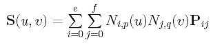
Let the desired B-spline surface of degree (p,q) defined by the unknown (e+1)×(f+1) control points P_ij's is the following:

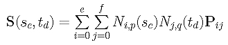
Because there are m+1 rows of data points, we need m+1 parameters in the u-direction, s₀, s₀, ..., s_m. Similarly, we need n+1 parameters in the v-direction, t₀, t₀, ..., t_n. The computation of these parameters is discussed in Parameters and Knot Vectors for Surfaces. With these parameters in hand, the point on surface that corresponds to data point D_cd is computed as follows:

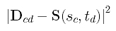
The squared error distance between D_cd and its corresponding point on surface is

The sum of all squared error distances is therefore the following:

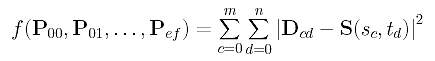
This is a function in the (e+1)×(f+1) unknown control points P_ij's. Similar to the case of global approximation, to minimize f(), we can compute the partial derivatives and set them to zero:

Then, we have (e+1)×(f+1) equations whose common zeros are the desired control points. Unfortunately, these equations are not linear and solving a system of non-linear equations is very time consuming. Rather than aiming for an optimal solution, we can find a reasonably good solution that does not minimize function f().

To find a non-optimal solution, we shall employ the same technique used in Global Surface Interpolation. More precisely, apply curve approximation to each column of data points to compute some "intermediate" data points. In this way, for each column of m+1 data points we compute e+1 "intermediate" data points. Since there are n+1 columns, these "intermediate" data points form a (e+1)×(n+1) grid. Then, apply curve approximation to each row of these intermediate data points to compute the desired control points. Since each row has n+1 "intermediate" data point and there are e+1 rows, each approximation for a row generates f+1 desired control points, and, as a result, we will finally obtain (e+1)×(f+1) control points. The following summarizes the required steps:

In this algorithm, n+1 curve approximations are applied to the columns of D's and then e+1 curve approximations are applied to the rows of the "intermediate" data points. Thus, n+e+2 curve approximations are performed. On the other hand, we could apply m+1 curve approximations to each row of the data points to create (m+1)×(f+1) "intermediate" data points. Then, f+1 curve approximations are applied to each column of this "intermediate" data points to obtain the final (e+1)×(f+1) control points. In this way, m+f+2 curve approximations are performed.

Since this algorithm does not minimize function f(), it is not an optimal one, although it is adequate for many applications.

Note that matrix N^T.N used in the first for loop does not change when going from column to column. Therefore, if we naively follow the above algorithm, we would end up solving the system of equation Q = (N^T.N)^.P n+1 times. This is, of course, not efficient. To speed up, the LU-decomposition of N^T.N should be computed before the first for loop starts, and the approximation in each iteration is simply a forward substitution followed by a backward substitution. Similarly, a new matrix N^T.N will be used for the second for loop. Its LU-decomposition should also be computed before the second for starts. Without doing so, we will perform (e+1)+(n+1)=e+n+2 LU-decompositions when only 2 would be sufficient.

A Simple Comparison

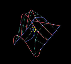
The following is a grid of six rows and five columns. We shall use it to illustrate the differences between interpolation and approximation. Images on the first column are the results before changing the indicated data points, while images on the second depict the results of this move.

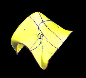
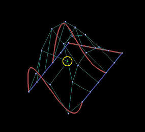
The first two rows show the results of global interpolation using the chord length method for determining parameters and knot vectors. The interpolating surface is of degree (3,3). The red and blue curves are knots curves (i.e., isoparametric curves at knots). The indicated data point changes its position slightly, but the blue knot curve changes its shape drastically. The difference between the two interpolating surfaces is even greater. Moving a data point to the right produces a large bulge in the left end of the surface. Moreover, a deep valley below the red knot curve is generated due to this move.

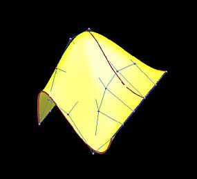
The last two rows show the results of global approximation. The number of control points in u- and v-directions are 5 and 4, respectively. It is obvious that the impact of changing the position of a data point on the shape of the approximation surface is not so dramatic. In fact, in this example, approximation is not so sensitive to changing the position of the indicated data point, and the approximation surfaces follow the shape of the data point net much better than those interpolating surfaces.

	Before Move	After Move
Int: Curve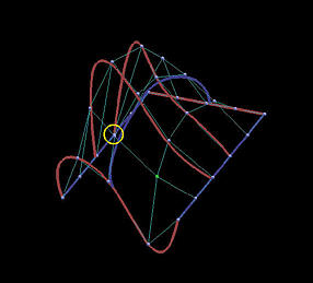
Int: Surface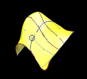
App: Curve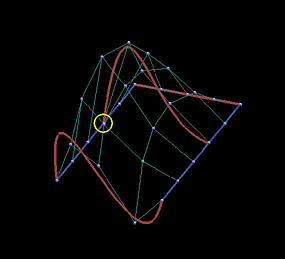
App: Surface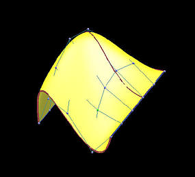