Introduction to Python

There are two main paths for coding in Python Jupyter notebooks either using your local machine or online resources. I will give instructions to install / set up either option.

There are many online Jupyter notebook resources that are free for educational uses including:

• Google's Colaboratory
• Deepnote
• and more

I will give information for Colaboratory or Colab.

Local Installation

Many of you will not have Python or associated libraries on your computer. Anaconda or conda is an easy way to install Python and create environments to manage the different Python versions and dependencies. This allows us to avoid conflicts between our preferred Python version and that used in other projects or classes.

1. Install Anaconda

Creating a Conda Environment

Once you have Anaconda installed, it makes sense to create a virtual environment for the course/project. If you choose not to use a virtual environment (strongly not recommended!), it is up to you to make sure that all dependencies for the code are installed globally on your machine.

Examples from [Anaconda Docs], starting from the default base environment.

To set up a virtual environment called py22, run the following in your terminal, press y to confirm any missing packages.

conda create --name py22 python=3.7

You can see a list of environments with:

conda info --envs 

Activating an Environment

To enter the conda environment that we just created, do the following. Note that the Python version within the environment is 3.7, just what we want.

conda activate py22

(py22) lebrown@lebrown-macbook web$ python -V
Python 3.7.10

Note, the tag (<env-name>) shows the name of the conda environment that is active.

Install Packages

Install packages you may / will need.

pip install pandas numpy scipy matplotlib seaborn scikit-learn 

This package installs several other packages we will use:

• numpy
• scipy
• pandas
• matplotlib
• seaborn
• scikit-learn
• ...

Deactivate an Environment

When you are done working on a project, leave the environment.

conda deactivate 

Online - Google Colaboratory

Colab short for (Colaboratory) is a new product by Google Research that allows data science, machine learning, and artificial intelligence students and researchers to work on projects in the browser. Like Google Docs or Sheets, it allows you to share projects between many people, and gives free access to GPUs to quickly train models.

Colab provides a cloud service based on Jupyter notebooks, combining notebooks and Google Drive. It comes with many packages preinstalled.

Note, you must have a Gmail account to use this tool.

Getting Started

Introduction adapated from Stanford's cs230 and 231n

Visit https://colab.research.google.com/. You should see something similar to below. Click the "Welcome to Colaboratory" to walk through some of the basics of a notebook.

This will bring you to a page like this, where some of the basic's of Colab can be introduced.

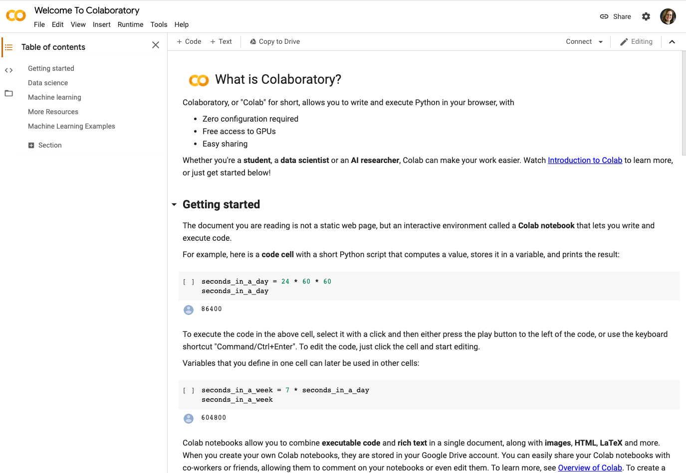
A notebook (Colab and Jupyter) is made up of cells. The cells can contain text, where you can describe what you are doing, and code, where you can enter Python code and run it.

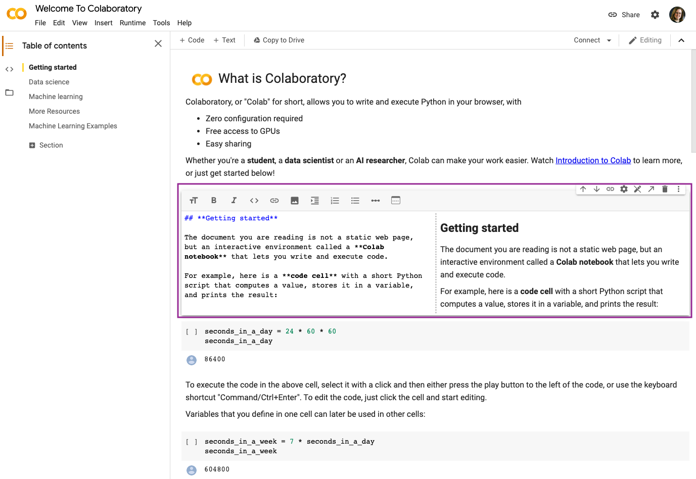
Text Cells

Here is an example of a text cell.

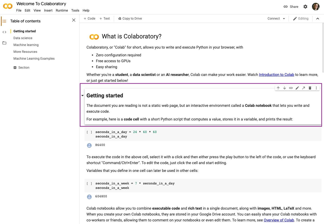
Double-clicking on the text cell allows you to edit. The text cells are formatted using Markdown. Markdown is a simple mark-up language that adds formatting to plain text. In Colab, you can also see a small interface to perform the text highlighting. We would recommend getting familiar with basic Markdown because it is easy to use and quicker to edit.

Markdown References

• Getting Started
• Syntax Guide
• Alternative Syntax Guide

Code Cells

The code cells contain Python code (Python 3.7).

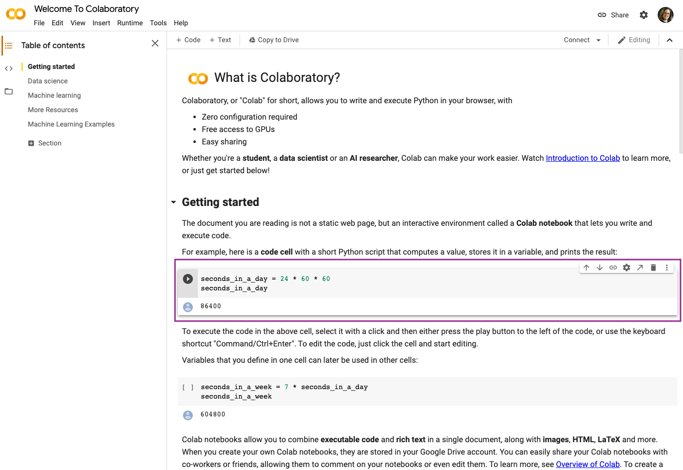
You can click in the code cell to edit the Python code. To execute/run the code you can click on the "play" icon, or by pressing CTRL + ENTER or ⌘ + ENTER. You can also use SHIFT + ENTER to run a code cell.

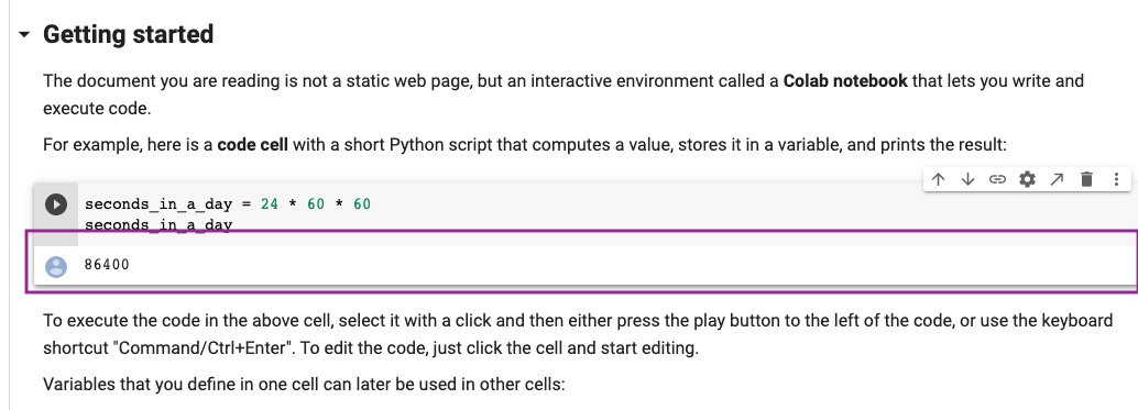
Output from the code cell appears below that cell. In this code block, the value of the variable seconds_in_a_day is printed.

Walk through the remaining information in the "Welcome" notebook.

User Interface

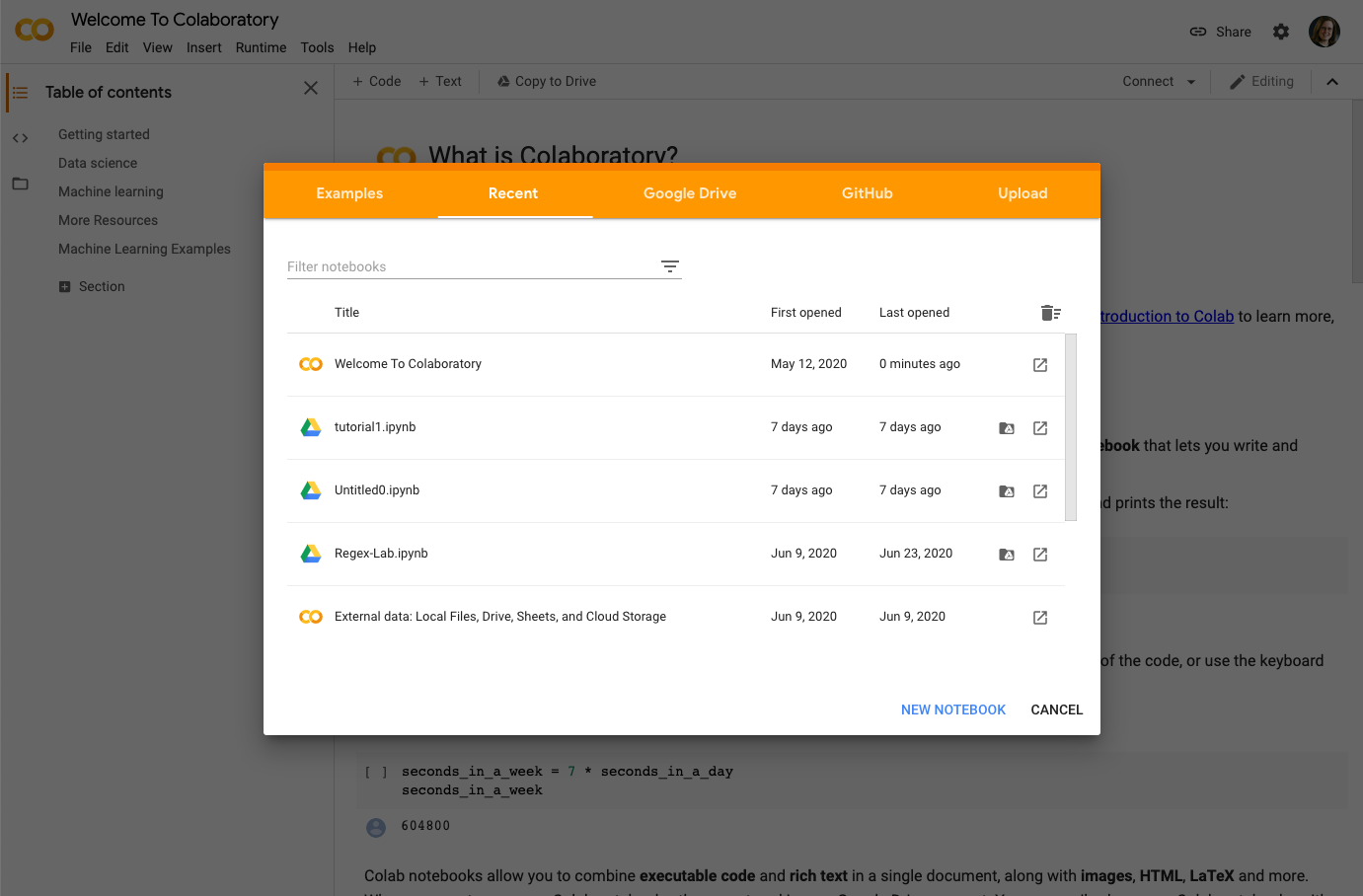
You can create a new notebook by clicking on File Menu (top left) -> New Notebook. Notice that there are options for opening different files and uploading files, these will be important for later.

Before we start getting into the coding, let's familiarize ourselves with the user interface (UI) of Google Colab.

What the different buttons mean:

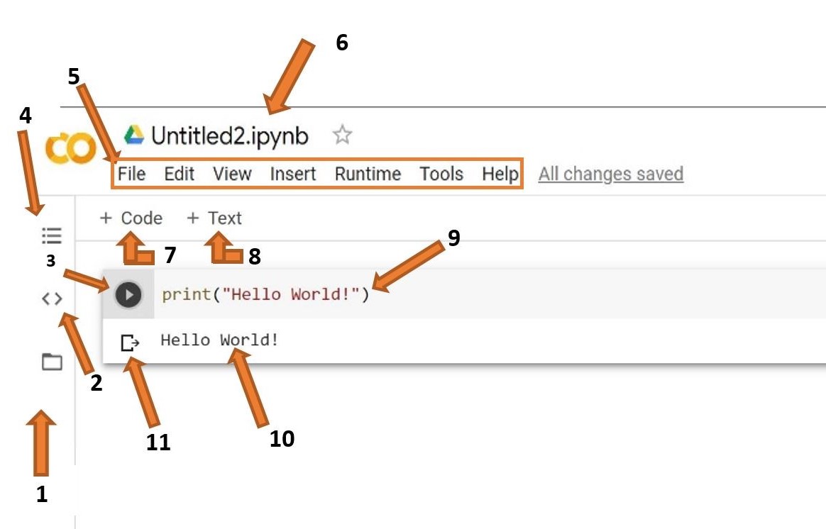
1. Files: Here you will be able to upload datasets and other files from both your computer and Google Drive
2. Code Snippets: Here you will be able to find prewritten snippets of code for different functionalities like adding new libraries or referencing one cell from another.
3. Run Cell: This is the run button. Clicking this will run any code that is inserted in the cell beside it. You can use the shortcut shift+enter to run the current cell and exit to a new one.
4. Table of Contents: Here you will be able to create and traverse different sections inside of your notebook. Sections allow you to organize your code and improve readability.
5. Menu Bar: Like in any other application, this menu bar can be used to manipulate the entire file or add new files. Look over the different tabs and familiarize yourself with the different options. In particular, make sure you know how to upload or open a notebook and download the notebook (all of these options are under "File").
6. File Name: This is the name of your file. You can click on it to change the name. Do not edit the extension (.ipynb) while editing the file name as this might make your file unopenable.
7. Insert Code Cell: This button will add a code cell below the cell you currently have selected.
8. Insert Text Cell: This button will add a text cell below the cell you currently have selected.
9. Cell: This is the cell. This is where you can write your code or add text depending on the type of cell it is.
10. Output: This is the output of your code, including any errors, will be shown.
11. Clear Output: This button will remove the output.
    
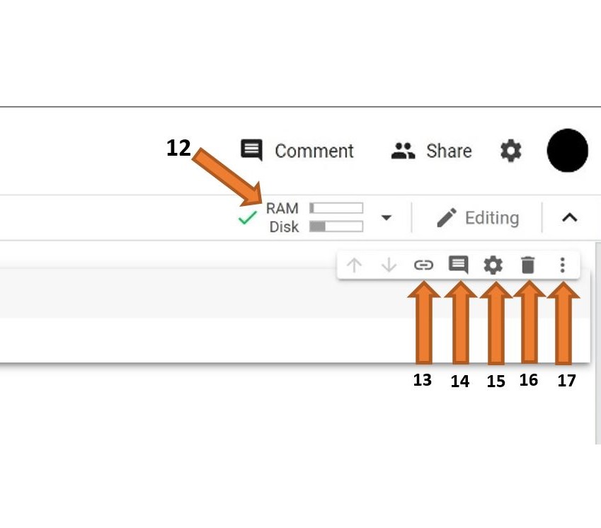
12. Ram and Disk: All of the code you write will run on Google's computer, and you will only see the output. This means that even if you have a slow computer, running big chunks of code will not be an issue. Google only allots a certain amount of Ram and Disk space for each user, so be mindful of that as you work on larger projects.
13. Link to Cell: This button will create a URL that will link to the cell you have selected.
14. Comment: This button will allow you to create a comment on the selected cell. Note that this will be a comment on (about) the cell and not a comment in the cell.
15. Settings: This button will allow you to change the Theme of the notebook, font type, and size, indentation width, etc.
16. Delete Cell: This button will delete the selected cell.
17. More Options: Contains options to cut and copy a cell as well as the option to add form and hide code.

Let's try something fun. Do the following: go to Settings(#15) -> Miscellaneous, check the boxes that say Corgi mode, and Kitty mode. Click save. Now wait a few seconds, keep an eye on the top of the web page. WARNING: Having this setting on might slow down your browser, so it is not recommended that you leave them on while working on assignments or projects.

Colab Code Cells

As you learned about Jupyter notebooks cells can contain either text written in Markdown or Python 3 code. Of course, this is true in Google Colab.

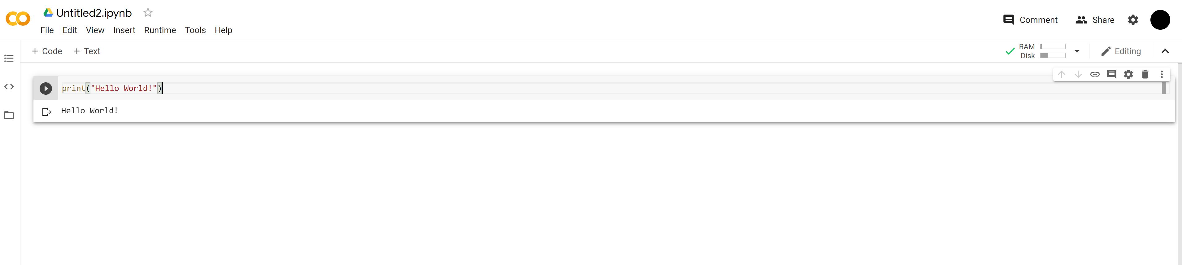
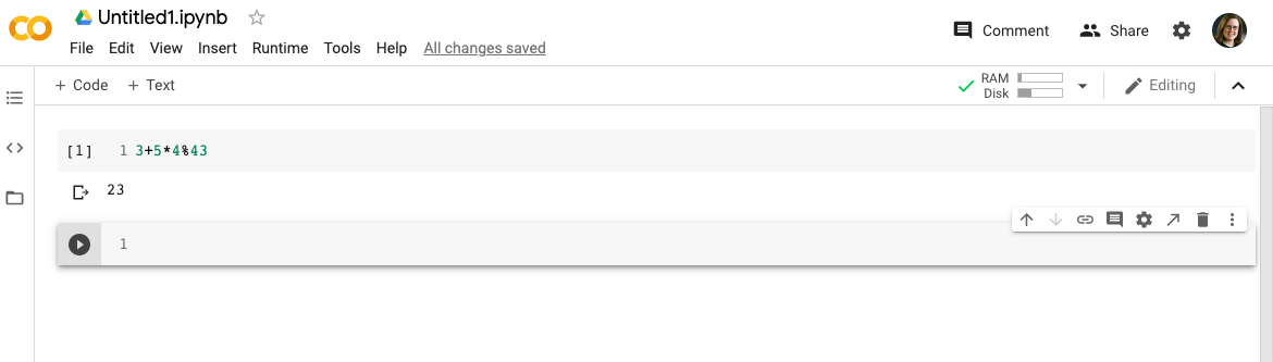
Clicking "run cell" on a code cell will execute the code in the cell. The output, if there is one, will be shown directly below the cell. In your notebook, copy the following code into a cell and running it.

3+5*4%43

Note, running the code the first time, can take a bit of time as the notebook connects up to resources. Here you can see the output of the code cell.

For each of the following bits of code, try copying and pasting the code into a new code cell (or typing the code into a code cell) then executing to see the results of the code.

Here we can run a more complicated bit of Python.

import math

circle_areas = []

for i in range(1, 5):
   circle_areas.append(math.pi * i**2)

circle_areas

Don't worry if you don't fully understand the code above, we will begin to walk you through Python next.

Notice that if the last line of a code cell is a value/variable, that value/variable will be printed in the output. If the last line is an assignment of a value to a variable, then nothing will be printed in the output. Alternatively, you may use a print statement, print (<variable name>), to see what is stored in the variable.

a = 5

Note that no output is produced when you run the above code cell. However, the value of "a" is saved and is available in other cells. Here we have included a print statement to show you what is stored in variable b.

b = a * a
print (b)

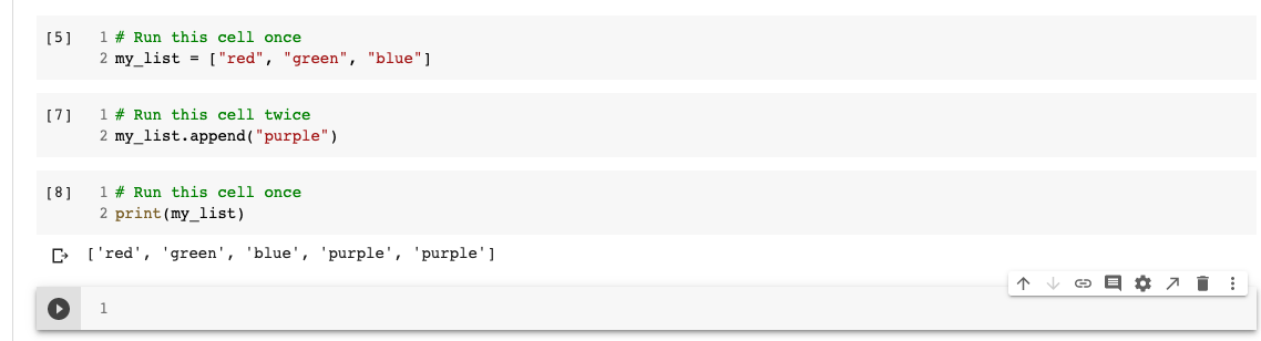
This is useful because it means that we can put "import" statements and the time-consuming reading of large data sources in one code cell usually at the start of the notebook, and you can experiment with manipulations of that data in later cells without having the wait to reload the data. The caveat to this is that each code cell is executed only when you run it, so you could accidentally or willfully run code cells out of order. Below is an example.

# Run this cell once
my_list = ["red", "green", "blue"]

# Run this cell twice
my_list.append("purple")

# Run this cell once
print(my_list)

Notice that my_list contains "purple" twice; even the code above only adds it once. In general, you should write your code assuming that each code cell is run once from top to bottom. There's even a menu to help you do that. The "Run" menu has "Run All Above Selected Cell" and "Run All Cells" functions that allow you to get your notebook in a predictable state if you ever get confused by having run cells multiple times or out of order.

You can see the order in which the code cells are run as it is printed in square brackets on the upper left corner of the code cell (in colab, when you hover the mouse on it, it turns into the execute arrow). Here, we can see that the cell starting with the comment # Run this cell once was the 5th cell run in the notebook. The following cell was run twice, then the cell containing the print statement was run (the 8th cell in the notebook).

Google Colab has preinstalled packages, modules, and libraries to make it easier for us to use it without worrying about having to import or install the packages ourselves. As you might have noticed in one of the code blocks above, "import math" allows you to utilize the math module which includes summation and subtraction. As you go further in this chapter, you will be importing other packages and libraries as well.

import pandas as pd
import numpy as np
import scipy as sc

Think of packages, libraries, and modules as separate files that exist outside of the one you are working on. They are an efficient part of programming so programmers don't have to re-write every bit of code from scratch. For instance, the math module already has addition and subtraction defined in it, so by importing it, you can build on top of it rather than having to reinvent the wheel.

The "import "statement tells the program that you are going to be referencing things that do not exist in this file. It also tells the program which file, among the files preinstalled in Colab, it is referring to. For example, import pandas as pd tells the program that you will be using things from the pandas "file" (package) and that whenever you type "pd" you are talking about the pandas package.

Saving Google Colab Notebooks

Now that you have created your first colab notebook you can save it. Similar to Google Docs or Sheets, you can click on the name at the top and save it, e.g., CADeT-welcome-notebook.ipynb.

You can download a copy of the notebook to your local machine using the "File -> Download .ipynb" command.

As a default, the colab notebook is stored in your Google Drive. There should be a new folder created in your drive called Colab Notebooks

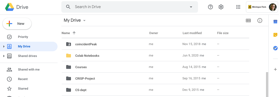
In the drive, you can create folders to organize your notebooks.

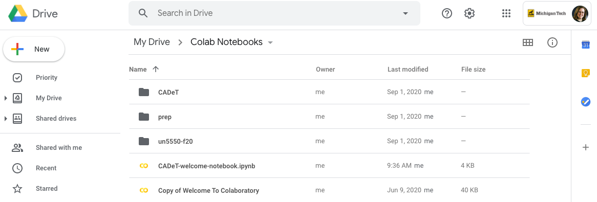
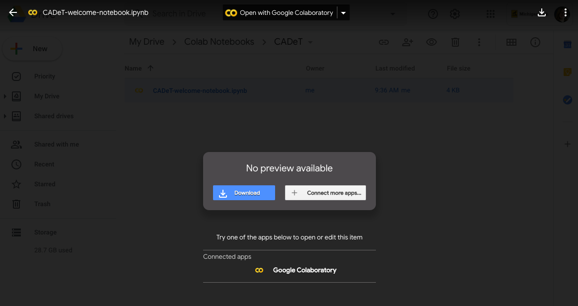
To open a notebook from the drive, double-click on it. You may encounter the following screen, where you will want to select to Open with Google Colaboraty from the top.