
Curve subdivision subdivides a curve at a point so that each of the two components posses the same type. Follow the procedure below to perform curve subdivision.
First, move the u-indicator to a place where you want to cut the curve. Select Techniques followed by Curve Subdivision. The original curve will be cut into two at the specified point.
Under this system, if a curve is subdivided at a particular u, the first curve segment has domain [0,u] and the second curve segment has domain [u,1]. After subdivision, the current curve is always the second one. The curve and its domain have the same color. You can always change the colors. See Changing the Color Scheme for the details.
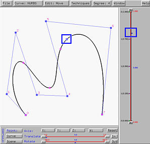
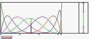
In the following figure, u is placed at 0.8. We intend to cut the curve at u = 0.8 into two sub-curves.
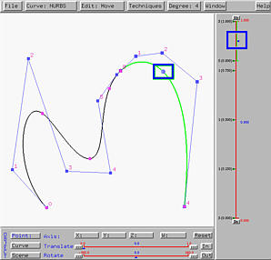
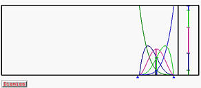
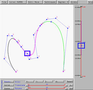
Select Techniques followed by Curve Subdivision. The result is shown in the left figure below. The two curve segments are shown in black and yellow. Note that your system may use different colors. As mentioned earlier, the second segment is always the current curve. As the u-indicator moves to [0.8,1], the sub-interval of the vertical slider is shown in the same color as that of the curve. Keep in mind that the current curve is always thicker and shown in brighter color. The right figure below is the partition of unity of this curve segment. Please note that the domain is [0.8,1].
If you slide the u-indicator down to a location less than 0.8, the current curve will automatically switch to the first curve segment, in this case, the black one. The domain of the current curve on the vertical slider is also shown in black, and the partition of unity window will show that of the current curve.
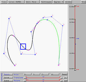
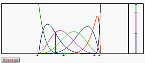
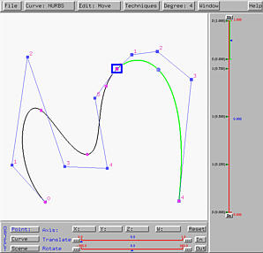
A subdivided curve can be further subdivided. For example, if the curve segment defined on [0,0.8] is further subdivided at u = 0.3, we have the left figure below. The black curve segment is the one on [0,0.3], while the blue one is the curve segment on [0.3,0.8]. Since this subdivision has no impact on the curve segment defined on [0.8,1], the yellow curve is the same as in the above figure.

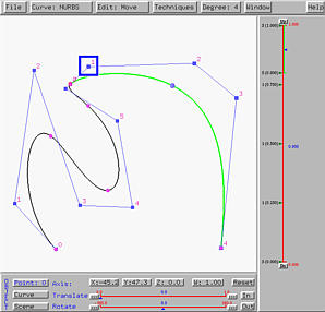
Let us move the common control point, the one marked with a blue rectangle, to a new place. The result is shown in the left figure below. As you can see, this system moves the common control point as well as its two adjacent neighbors. Therefore, the curve segments are still tangent to the line segment at the common control point.
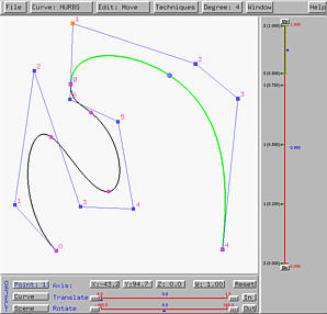
Let us now move one of the two neighbors of the common control point, say the one marked with a blue rectangle in the left figure above. Once that control point is moved, the control point at the other end will also move. In face, these two control points will rotate about the common control points to keep these three control points collinear. Moreover, the length between this endpoint and the common point will be adjusted to maintain C1-continuity. A result is shown in the right figure above.