
Surface subdivision is a technique for subdividing a given surface patch along an isoparametric curve into two subpatches, each of which receives its own control points, knot vectors and degree. The boundary curve of the two subpatches is generated from the same set of control point, the same knot vector and the same degree.
Surface subdivision can be performed on the u- or the v- direction. To perform a subdivision, one should move the uv-indicator and select subdivision. Then, the surface will be subdivided along the current u or v value. We shall use a NURBS surface defined by 6 rows and 6 columns of control points and degrees 4 and 3 in the u- and the v- direction, respectively. You can click here to download a copy of this file deg-elev.dat for your practice. Note that this file is also used in the discussion of degree elevation.
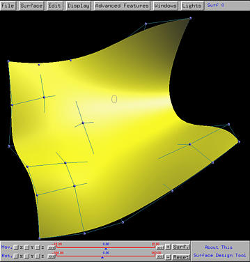
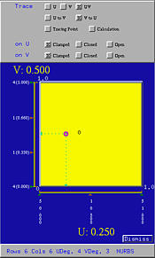
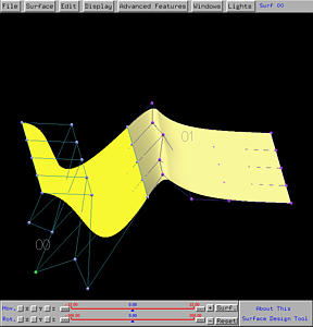
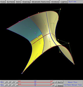
The following shows the surface. Suppose we want to subdivide this surface along the isoparametric curve at u = 25. The first thing to do is to move the uv-indicator to a position with a u value being 0.25. The v value has no effect. Note that we also use Display followed by Show Surface IDs. Thus, the only displayed surface has an ID 0.
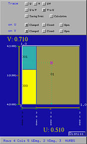
Select Advanced Features, followed by Surface Subdivision, followed by on U. The given surface is subdivided into two subpatches with different colors. The surface domain in the Tracing Window is also subdivided at u = 0.25. Now, we shall learn something about the surface ID naming scheme. Suppose a surface k is subdivided into two. The two subpatches will receive IDs k0 and k1, with k0 being assigned to the original patch. The original ID k is no more used. Thus, if subpatch k1 is subdivided again into two smaller patches, their surface IDs are k10 and k11. In this way, you can quickly identify where a subpatch comes from.
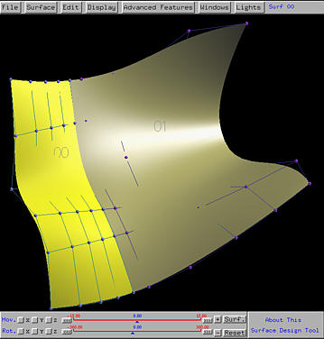
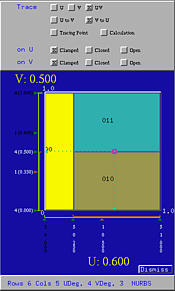
All subpatches share the original domain [0,1]×[0,1]. In the above, surface 00 has domain [0,0.25]×[0,1], while surface 01 has domain [0.25,1]×[0,1]. Isoparametric curve along u = 0.25 is the common boundary. Also note that the knots in the u-direction are modified. When the uv-indicator moves into the domain of a subpatch, the knots of this subpatch are shown in white color; those knots do not belong to this subpatch are shown in black. By the way, you can click the domain of a subpatch to select it, making it the current surface.
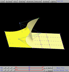
Please note that the control points of the boundary curve of the two subpatches are identical.
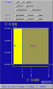
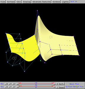
If we want to subdivide surface 01 into two subpatch along the isoparametric curve v = 0.5, then we can drag the uv-indicator to the domain marked with 01 until the value of v becomes 0.5. Select Advanced Features, followed by Surface Subdivision, followed by on V. Then, surface 01 is subdivided into surface 010 and 011.
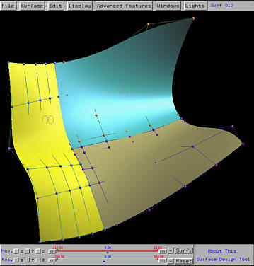
From the above figure, we still see the control points of the boundary curve between surfaces 010 and 011 are identical. However, since the boundary curve between surfaces 00 and the original 01 is subdivided, the boundary curve between 00 and 010 and the boundary curve between 00 and 011 are two subcurve of the original. As a result, control points do not have a one-to-one correspondence. More precisely, the boundary curve segment between 00 and 010 are defined by two different sets of control points. The same happens to the boundary curve between 00 and 011.

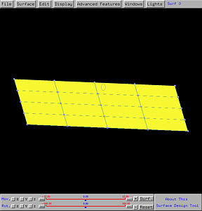
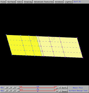
We shall use a planar surface to illustrate this effect. Click here to download file plane.dat for your practice. The generated surface is shown in the left figure below. The right figure shows the subdivision in the u-direction at u = 0.4.
Select Advanced Features, followed by Surface Subdivision, followed by Enable Maintaining C1. This will enable the system to maintain C1 continuity. Then, moving the control points next to the boundary control points will guarantee the two subpatches to join smoothly (see the left figure below). On the other hand, selecting Disable Maintaining C1 will disable this feature. In this case, moving control points next to the boundary control points will destroy this smoothness as shown in the right figure below. More precisely, sharp angle or folding may occur.
When Enable Maintaining C1 is in effect, moving control point Pk0 will cause the other control point Pk1 to move accordingly to maintain this smoothness. As a result, to adjust the shape of a subdivided surface, moving either Pk0 or PK1 would be sufficient.
Note that moving boundary control points will destroy the C1 continuity since this version does not support this feature. It will be available in next version. Start with the same surface and subdivide it at u = 0.4. The following figure shows the effect of moving those control points on the boundary even if Enable Maintaining C1 is in effect. A ridge is clearly shown.

What if you want to apply a display option to all subpatches of a surface? One way to do that is selecting each subpatch in turn and turn on/off the desired display option. There is a simpler way. Select Edit, followed by Display Globally. Then, most display options selected will be applied to all subpatches. For example, if we choose Select Edit, followed by Show Control Points, Show Control Net, and Show Knot Curves, all three options apply to the surface as shown below. Now, every subpatch is displayed with control points, control net and knot curves.
If you select Edit, followed by Display Locally, all subsequent display options will only affect the current subpatch (i.e., the subpatch corresponds to the domain that currently contains the uv-indicator).