Curve Global Approximation

In interpolation, the interpolating curve passes through all given data points in the given order. As discussed on the Global Interpolation page, an interpolating curve may wiggle through all data points rather than following the data polygon closely. The approximation technique is introduced to overcome this problem by relaxing the strict requirement that the curve must contain all data points. In global approximation, except for the first and last data points, the curve does not have to contain every point.

To measure how well a curve can "approximate" the given data polygon, the concept of error distance is used. The error distance is the distance between a data point and its "corresponding" point on the curve. Thus, if the sum of these error distances is minimized, the curve should follow the shape of the data polygon closely. An interpolating curve is certainly such a solution because the error distance of each data point is zero. However, the formulation to be discussed is unlikely to yield an interpolating curve. A curve obtained this way is referred to as an approximation curve.

Suppose we are given n+1 data points D₀, D₁, ..., D_n, and wish to find a B-spline curve that follows the shape of the data polygon without actually containing the data points. To do so, we need two more input: the number of control points (i.e., h+1) and a degree (p), where n > h >= p >= 1 must hold. Thus, approximation is more flexible than interpolation, because we not only select a degree but also the number of control points. The following is a summary of our problem:

Global Curve Approximation
Given a set of n+1 data points, D₀, D₁, ..., D_n, a degree p, and a number h, where n > h >= p >= 1, find a B-spline curve of degree p defined by h+1 control points that satisfies the following conditions:

this curve contains the first and last data points (i.e., D₀ and D_n) and

this curve approximates the data polygon in the sense of least square.

With h and p in hand, we can determine a set of parameters and a knot vector. Let the parameters be t₀, t₁, ..., t_n. Note that the number of parameters is equal to the number of data points. Now, suppose the approximation B-spline of degree p is

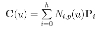
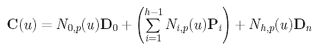
where P₀, P₁, ..., P_h are the h+1 unknown control points. Since we want the curve to pass the first and last data points, we have D₀ = C(0) = P₀ and D_n = C(1) = P_h. Therefore, there are only h - 1 unknown control points P₁, P₂, ..., P_h-1. Taking this into consideration, the curve equation becomes the following:

The Meaning of Least Square

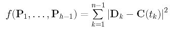
How do we measure the error distance? Because parameter t_k corresponds to data point D_k, the distance between D_k and the corresponding point of t_k on the curve is |D_k - C(t_k)|. Since this distance consists of a square root which is not easy to handle, we choose to use the squared distance |D_k - C(t_k)|². Hence, the sum of all squared error distances is

Our goal is, of course, to find those control points P₁, ..., P_h-1 such that the function f() is minimized. Thus, the approximation is done in the sense of least square.

Finding a Solution

This section is a little messy and requires some knowledge in linear algebra. First, let us rewrite D_k - C(t_k) into a different form:

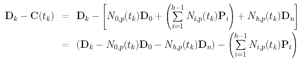
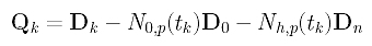
In the above, D₀, D_k and D_n are given, and N_0,p(t_k) and N_h,p(t_k) can be obtained by evaluating N_0,p(u) and N_h,p(u) at t_k. Click here to learn how to compute these coefficients. For convenience, let us define a new vector Q_k as:

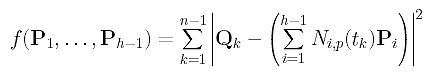
Then, the sum-of-square function f() can be written as follows:

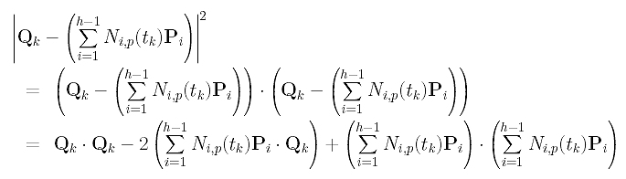
Next, we shall find out what the squared error distance looks like. Recall the identity x^.x = |x|². This means the inner product of vector x with itself gives the squared length of x. Thus, the error square term can be rewritten as

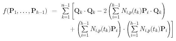
Then, function f() becomes

How do we minimize this function? Function f() is actually an elliptic paraboloid in variables P₁, ..., P_h-1. Therefore, we differentiate f() with respect to each P_g and find the common zeros of these partial derivatives. These zeros are the values at which function f() attends its minimum.

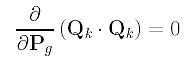
In computing the derivative with respect to P_g, note that all Q_k's and N_i,p(t_k) are constants (i.e., no P_k involved) and their partial derivatives with respect any P_g must be zero. Therefore, we have

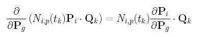
Consider the second term in the summation, which is the sum of N_i,p(t_k)P_i ^.Q_k's. The derivative of each sub-term is computed as follows:

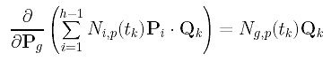
The partial derivative of P_i with respect to P_g is non-zero only if i = g. Therefore, the partial derivative of the second term is the following:

The derivative of the third term is more complicated; but it is still simple. The following uses the multiplication rule (f^.g)' = f'^.g + f^.g'.

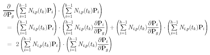
Since the partial derivative of P_i with respect to P_g is zero if i is not equal to g, the partial derivative of the third term in the summation with respect to P_g is:

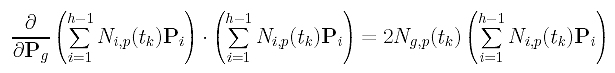
Combining these results, the partial derivative of f() with respect to P_g is

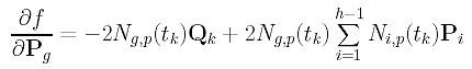
Setting it to zero, we have the following:

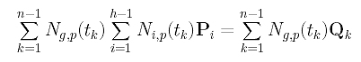
Since we have h-1 variables, g runs from 1 to h-1 and there are h-1 such equations. Note that these equations are linear in the unknowns P_i's. Before we go on, let us define three matrices:

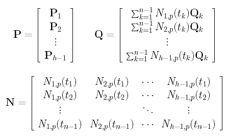
Here, the k-th row of P is the vector P_k, the k-th row of Q is the right-hand side of the k-th equation above, and the k-th row of N contains the values of evaluating N_1,p(u), N_2,p(u), ..., N_h-1,p(u) at t_k. Therefore, if the input data points are s-dimensional vectors, P, N and Q are (h-1)×s, (n-1)×(h-1) and (h-1)×s matrices, respectively.

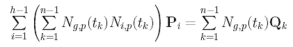
Now, let us rewrite the g-th linear equation

into a different form so that the coefficient of P_i can easily be read off:

Finally, the coefficient of P_i is

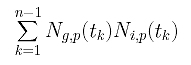
If you look at matrix N, you should see that N_g,p(t₁), N_g,p(t₂), ..., N_g,p(t_n-1) are the g-th column of N, and N_i,p(t₁), N_i,p(t₂), ..., N_i,p(t_n-1) are the i-th column of N. Note that the g-th column of N is the g-th row of N's transpose matrix N^T, and the coefficient of P_i is the "inner" product of the g-th row of N^T and the i-th column of N. With this observation, the system of linear equations can be rewritten as

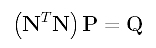
Since N and Q are known, solving this system of linear equations for P yields the desired control points. And, of course, we have found the solution.

An Algorithm

Although the development in the previous section is lengthy and tedious, the final result is surprisingly simple: solving a system of linear equations just like we encountered in global interpolation. As a result, the algorithm for global approximation is also quite simple.

Input: n+1 data points D₀, D₁, ..., D_n, a degree p, and the desired number of control points h+1;
Output: A B-spline curve of degree p, defined by h+1 control points, that approximates the given data points;
Algorithm:
Obtain a set of parameters t₀, ..., t_n and a knot vector U;
Let P₀ = D₀ and P_h = D_n;
for k := 1 to n-1 do

Compute Q_k with the following formula:
for i := 1 to h-1 do

Compute the following and save it to the i-th row of matrix Q;
/* matrix Q is available */
for k := 1 to n-1 do

for i := 1 to h-1 do

Compute N_i,p(t_k) and save to row k and column i of N;

/* matrix N is available */
Compute M = N^T^.N;
Solving for P from M^.P = Q;
Row i of P is control point P_i;
Control points P₀, ..., P_h, knot vector U and degree p determines an approximation B-spline curve;

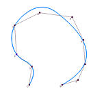
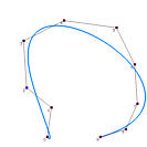
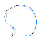
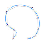
The Impact of Degree and Number of Control Points

It is obvious that the data points affect the shape of the approximation curve. What is the impact of degree p and the number of control points on the shape of the curve? The following figures show some approximation curves for 10 data points (n=9) with various degrees and numbers of control points. Each row gives the approximation curves of the same degree but with different number of control points, while each column shows the same number of control points with different degree. Note that all curves use the centripetal method for computing its parameters.

	Points = 4	Points = 5	Points = 6	Points = 7
Deg 2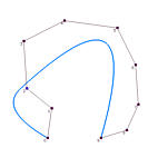
Deg 3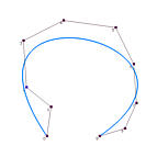
Deg 4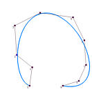
Deg 5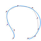

It is understandable that lower degree curves in general will not be able to approximate the data polygon well because they are not very flexible. Therefore, on each column, higher degree curves yield better results (i.e., closer to the data polygon). By the same reason, more control points offer higher flexibility of the approximation curve. Hence, on each row, as the number of control points increases, the curve becomes closer to the data polygon.

Shall we use higher degree curves and many control points? The answer is no because global approximation may use fewer number of control points than global interpolation. If the number of control points is equal to the number of data points, global approximation becomes global interpolation, and we can just use global interpolation! As for degree, we certainly want the smallest one as long as the produced curve can capture the shape of the data polygon.

Why Is This Method Global?

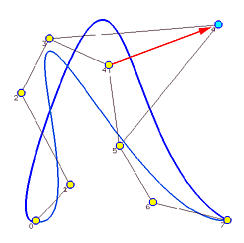
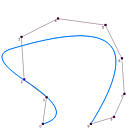
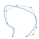
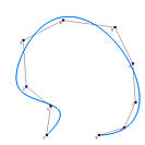
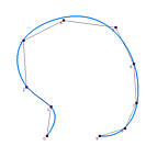
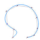
This approximation method is global because changing the position of a data point causes the entire curve to change. The yellow dots in the following image are the given data points to be approximated by a B-spline curve of degree 3 and 5 control points (i.e., n = 7, p=3 and h = 4). The parameters are computed with the centripetal method. Suppose data point 4 is moved to a new position indicated by a light blue dot. The new approximation B-spline is the one in blue color. As you can see, except for the first and last data points which are fixed by the algorithm, the shapes of the original curve and the new one are very different. Therefore, changes due to modifying data points are global!