The Universal Method

In 1999 Choong-Gyoo Lim proposed an interesting method for selecting parameters. In previously discussed methods, we determine the parameters and then generate a knot vector. Lim's method, known as the universal method, works the other way around by using uniformly spaced knots for computing the parameters.
Suppose we need n+1 parameters, one for each data points, and the degree of the desired interpolating B-spline curve is p. Then, the number of knots is m+1, where m = n + p + 1. Lim suggested that these knots should be uniformly spaced. More precisely, the first p+1 knots are set to 0, the last p+1 knots are set to 1, and the remaining n - p knots evenly subdivide the domain [0,1]. Therefore, the knots are:
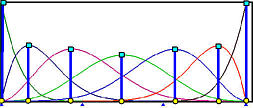
This set of clamped type knots defines n+1 B-spline basis functions. Then, the parameters are chosen to be the values at which their corresponding basis functions reach a maximum. Take a look at the following figure, where n = 6 (i.e., 7 data points), p = 4, and m = 11 (i.e., 12 knots). Because we use clamped knots, 0 and 1 are two knots of multiplicity 5 (i.e., p+1) and there are only two internal knots at 1/3 and 2/3. Note that there are n+1 B-spline basis functions, and the maximums of the first and the last are 0 and 1, respectively. The other maximums are marked with blue bars, and the parameters are marked with yellow dots.
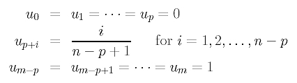
Let us do a hand calculation example. Suppose we have 4 data points (i.e., n=3) and degree p=2. Thus, the number of knots is 7 (i.e., m = n + p + 1 = 6). Since the knots are uniformly spaced, they are
| u0 = u1 = u2 | u3 | u4 = u5 = u6 |
| 0 | 0.5 | 1 |
Then, we can compute the desired B-spline Basis functions. Let us start with degree 0 (i.e., p = 0). Click here to review the definition of B-spline basis functions, and here for computation examples. The computed results are:
| Knot span | Basis Function |
| [u0,u1) = [0,0) | N0,0(u) = 0 |
| [u1,u2) = [0,0) | N1,0(u) = 0 |
| [u2,u3) = [0,0.5) | N2,0(u) = 1 |
| [u3,u4) = [0.5,1) | N3,0(u) = 1 |
| [u4,u5) = [1,1) | N4,0(u) = 0 |
| [u5,u6) = [1,1) | N5,0(u) = 0 |
Next, we compute basis functions of degree 1. Since N0,0(u) and N1,0(u) are both 0, N0,1(u) is zero everywhere. Similarly, N4,1(u) is also zero everywhere. Therefore, for basis functions of degree 1, we only need to compute N1,1(u), N2,1(u) and N3,1(u) as shown below:
| Basis Function | Equation | Non-zero Range |
| N0,1(u) | 0 | everywhere |
| N1,1(u) | 1-2u | [0,0.5) |
| N2,1(u) | 2u | [0,0.5) |
| 2(1-u) | [0.5,1) | |
| N3,1(u) | 2u-1 | [0.5,1) |
| N4,1(u) | 0 | everywhere |
The basis functions of degree 2 are computed as follows:
| Basis Function | Equation | Non-zero Range |
| N0,2(u) | (1-2u)2 | [0,0.5) |
| N1,2(u) | 2u(2-3u) | [0,0.5) |
| 2(1-u)2 | [0.5,1) | |
| N2,2(u) | 2u2 | [0,0.5) |
| -2(1-4u+3u2) | [0.5,1) | |
| N3,2(u) | (2u-1)2 | [0.5,1) |
The following figure shows all four B-spline basis functions of degree 2.
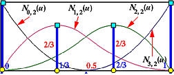
It is not difficult to verify that the maximums of N0,2(u), N1,2(u), N2,2(u) and N3,2(u) are 1 at u = 0, 2/3 at u = 1/3, 2/3 at u = 2/3 and 1 at u = 1. Therefore, with the universal method, the knot vector is { 0, 0, 0, 0.5, 1, 1, 1} and the parameter vector is { 0, 1/3, 2/3, 1}. We have a uniformly spaced parameter in this case. However, the parameters are not necessarily uniformly spaced in general, although the distribution of parameters is usually very even. Because of this fact, the universal method performs like the uniformly spaced method.
Because the knots are uniformly spaced, there is no multiple knots and all basis functions are of Cp-1 continuous. Click here to learn more about continuity of B-spline basis functions. Therefore, in practice, the maximum of a B-spline basis function does not have to be computed precisely. Our experience shows that sampling some values in the non-zero domain and choosing the one with maximum function value usually provides rather accurate result. If accurate maximums are desirable, one-dimensional search techniques such as the Golden Section Search can be used. The search domain is, of course, the non-zero domain of a B-spline basis function.
The universal method has a very interesting property. That is, it is affine invariant. This means, the transformed interpolating B-spline curve can be obtained by transforming the data points. This is similar to the affine invariance property of B-spline curves. In fact, it can easily be shown that if the same set of knots and parameters are used in the original and transformed interpolating B-spline curves, then transforming the curve can be achieved by transforming the data points. From this result, we immediately know that the uniformly spaced method is affine invariant, because the knot vector is computed from a set of uniformly spaced parameters which are not changed before and after a transformation. However, the chord length method and centripetal method are not affine invariant, because in the transformed curve, the distribution of chord lengths may not be the same as the original. As a result, after transforming the data points, we have a new set of chord lengths from which a new set of parameters must be computed.