|
|
|
| (a) | (b) | (c) |
|
|
| (d) | (e) |

De Boor's algorithm is a generalization of de Casteljau's algorithm. It provides a fast and numerically stable way for finding a point on a B-spline curve given a u in the domain.
Recall from a property of multiple knots that increasing the multiplicity of an internal knot decreases the number of non-zero basis functions at this knot. In fact, if the multiplicity of this knot is k, there are at most p - k + 1 non-zero basis functions at this knot. Consequently, at a knot of multiplicity p, there will be only one non-zero basis function whose value at this knot is one because of the property of partition of unity. Let this knot be ui. If u is ui, since Ni,p(u) is non-zero on [ui,ui+1), the point on the curve C(u) is affected by exactly one control point Pi. More precisely, we actually have C(u) = Ni,p(u) Pi = Pi!
So, what is the point of this interesting or somewhat strange property? Simple: if a knot u is inserted repeatedly so that its multiplicity is p, the last generated new control point is the point on the curve that corresponds to u. Why is this so? After inserting u multiple times, making its multiplicity p, the triangular computation scheme yields one point. Because the given B-spline curve must pass this new point, it is the point on the curve corresponding to u. This observation provides us with a technique for finding C(u) on the curve. We just insert u until its multiplicity becomes p and the last point is C(u)!
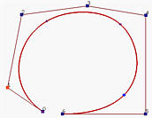
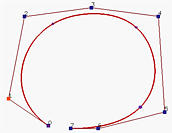
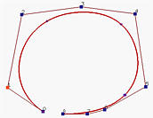
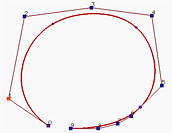
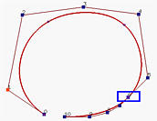
Let us take a look at an example before move on. Figure (a) is a B-spline curve of degree 4 defined by 7 control point. To compute C(0.9), where 0.9 is not a knot, u = 0.9 is inserted 4 (the degree) times. Figure (b) and Figure (c) show the results after the first and second insertion. Thus, two new control points are added near the lower right corner. Note that the control polyline is closer to the curve than the original. The result of the third insertion is shown in Figure (d). The fourth insertion yields the point on the curve (Figure (e)). Therefore, after four insertions, C(0.9) is a control point.

|

|

|
| (a) | (b) | (c) |

|

|
| (d) | (e) |
The general knot insertion algorithm discussed on the previous page can easily be modified to fulfill our purpose. First note that we only need to insert u enough number of times so that u becomes a knot of multiplicity p. If u is already a knot of multiplicity s, then inserting it p - s times would be sufficient.
In the left diagram below, all Pi,0's are on the left column. From the 0-th column and coefficients ai,1, one can compute Pi,1's. From this first column and coefficients ai,2's, the second column is computed and so on. Since there are (k-s)-(k-p)+1 = p-s+1 points on the zero-th column and since each column has one point less than the previous one, it takes p-s columns to reduce the number of points on a column to 1. This is why the last point is Pk-s,p-s. The right diagram shows the corner-cutting process.
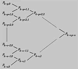
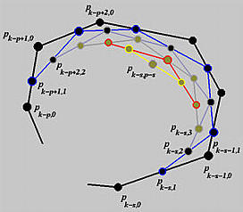
Although this process looks like the one obtained from de Casteljau's algorithm, they are very different. First, under de Casteljau's algorithm, the dividing points are computed with a pair of numbers 1 - u and u that never change throughout the computation procedure, while under de Boor's algorithm these pairs of numbers are different and depend on the column number and control point number. Second, in de Boor's algorithm only p+1 affected control points are involved in the computation, while de Casteljau's algorithm uses all control points. Since control points Pk-p to Pk define a convex hull that contains the curve segment on knot span [uk, uk+1), the computation of de Boor's algorithm is performed within the corresponding convex hull.

| u0 = u1 = u2 = u3 | u4 | u5 | u6 | u7 = u8 = u9 = u10 |
| 0 | 0.25 | 0.5 | 0.75 | 1 |
Based on this information, we shall compute P(0.4). For de Boor's algorithm, this is equivalent to inserting u = 0.4 three times. Since u = 0.4 is not an existing knot, s = 0 and u = 0.4 is in [u4, u5), the affected control points are P4, P3, P2 and P1. The following is the computation scheme:
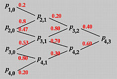
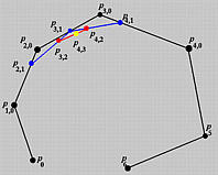
Let us compute the second column. The involved a coefficients are
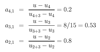
The first column is computed as follows:

To compute the second column, we need the following coefficients:
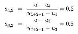
The points are

Finally, since

the final point is

This is the point on the curve corresponding to u = 0.4.
Notice the similarity of the intermediate polylines generated by de Boor's algorithm and those generated by de Casteljau's algorithm. Also note that u is not a knot in this example. If u is a knot, the computation will be easier since we will have fewer number of affected control points.