
Subdividing a B-spline curve follows exactly the same procedure for subdividing a Bézier curve. However, de Boor's algorithm will be used.
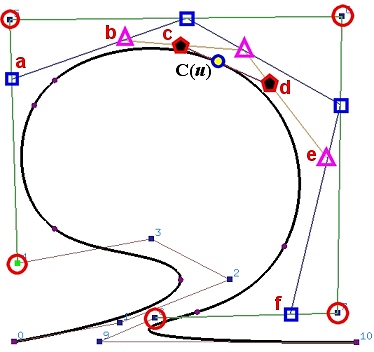
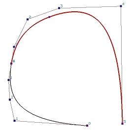
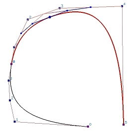
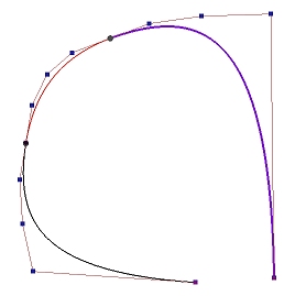
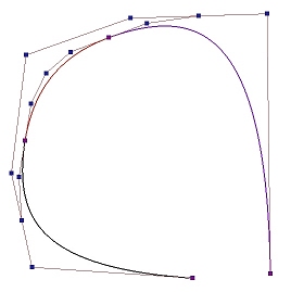
The following shows a B-spline curve of degree 3 defined by 11 (n = 10) control points. Suppose we wish to subdivide this curve at u = 0.5. The computation process of C(0.5) using de Boor's algorithm generates a de Boor net. In the figure below, points on column 0 are marked with circles, points on column 1 are marked with squares, points on column 2 are marked with triangles, points on column 3 are marked with pentagons, and the point on the curve C(u) is on column 4. Therefore, the control points of the B-spline curve on [0,u] are P0, P1, P2, P3, P4, a (take a turn), b (take a turn), c (take a turn), and C(0.5). The control points of the B-spline curve defined on [u,1] are C(0.5), d (take a turn), e (take a turn), f (take a turn), P8, P9 and P10.

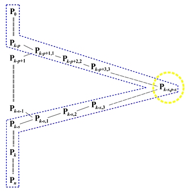
Thus, the control points for the curve on [0,u] include the original unaffected control points and the first point of each polyline of the de Boor net. Similarly, the control points for the curve on [u,1] consists of the last point of each polyline of the de Boor net, followed by the other unaffected control points. Since the first and last points of a polyline of a de Boor net are the first and last points on the same column, they can be extracted once a column is completely computed.
In the following diagram showing the triangular computation scheme of de Boor's algorithm, we can immediately extract Pk-p (curve on [0,u]) and Pk-s (curve on [u,1]). Once column 1 is computed, we can extract Pk-p+1,1 (curve on [0,u]) and Pk-s,1 (curve on [u,1]). After column 2 is computed, we can extract Pk-p+2,2 (curve on [0,u]) and Pk-s,2 (curve on [u,1]). This process continues until we reach Pk-s,p-s = C(u) which will be selected for both curves. Thus, graphically, points on the upper edge of the wedge from P0 to Pk-s,p-s form the control points of the curve on [0,u], and points on the lower edge from Pk-s,p-s to Pn form the control points of the curve on [u,0].
For example, if the original knot vector of a B-spline curve of degree 4 is { 0(5), 0.3, 0.4, 0.6, 0.7, 0.85, 0.9, 1(5) }. If the curve is divided at u = 0.65, the curve on [0,0.65] has a knot vector { 0(5), 0.3, 0.4, 0.6, 0.65(5) } and the curve on [0.65, 1] has a knot vector { 0.65(5), 0.7, 0.85, 0.9, 1(5) }.
It can be shown that the component curves constructed this way are also B-spline curves with the original degree and are part of the original curve on [0,u] and [u,1].

|
|
|
| (a) | (b) | (c) |
|
|
|
| (d) | (e) | (f) |
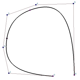
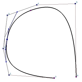
Why is each segment a Bézier curve? Since the given B-spline curve is subdivided at its knots, each curve segment has no internal knots. Moreover, the subdivision process makes the internal knots to have multiplicity p+1, and the curve segment is "clamped" at the first and last control points of each curve segment. From a previous page, we know that these curve segments must be Bézier curves.
In the process of subdividing a B-spline curve, a large number of control points will be introduced. Therefore, manipulating a B-spline curve is easier than manipulating its component Bézier curves. Moreover, the B-spline curve is Cp-k continuous at a knot point, where k is the multiplicity of the corresponding knot. When we manipulate a B-spline curve by moving control points, this continuity is always maintained. However, if a B-spline curve is subdivided into a sequence of Bézier curves, maintaining the continuity at the joining control points would be a challenging task. Consequently, handling a B-spline curve is much easier than handling a sequence of Bézier curves.