Rational Bézier Curves

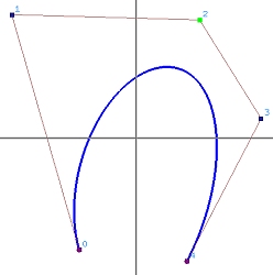
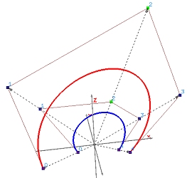
We have learned that projecting a 4-dimensional B-spline curve to hyperplane w=1 yields a 3-dimensional NURBS curve. What if this B-spline curve is a Bézier curve? The result is a Rational Bézier curve! The left image below shows a rational Bézier curve of degree 4, and the right one shows the relationship between a 3-dimensional Bézier curve of degree 4 (in red) and its projection rational Bézier curve (in blue) in hyperplane w=1.

What is the curve defined by a set of n+1 control points P₀, P₁, ..., P_n, each of which is associated with a non-negative weight w_i (i.e., P_i has weight w_i >= 0), and knots 0 (multiplicity n+1) and 1 (multiplicity n+1)? Since the 4-dimensional B-spline curve defined by the lifted control points P^w_i (0 <= i <= n) reduces to a Bézier curve of degree n, its basis functions are B_n,0(u), B_n,1(u), ..., B_n,n(u). Projecting this Bézier curve to hyperplane w = 1, we have the following:

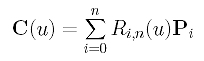
where R_i,n(u) is defined as follows:

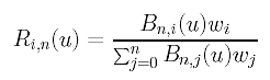
This is a special case of NURBS curves and is referred to as a rational Bézier curve. Since a rational Bézier curve is a special case of NURBS curves, rational Bézier curves satisfy all important properties that NURBS curves have. This is similar to the fact that Bézier curves have all the important properties of B-spline curves. However, since there is no internal knots, rational Bézier curves do not have the local modification property, which means modifying a control point or its weight will cause a global change. Moreover, the curve is now contained in the convex hull defined by the whole set of control points, and modifying the weight of a control point will push or pull the curve away from or toward the control point. Of course, rational Bézier curves are projective invariant rather than affine invariant! See NURBS: Important Properties for more details.