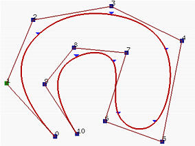
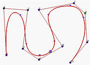
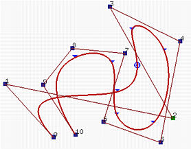
As mentioned in previous page, p(u) can be viewed as the union of curve segments defined on each knot span. In the figure below, where n = 10, m = 14 and p = 3, the first four knots and last four knots are clamped and the middle 7 knots are uniformly spaced. There are eight knot spans, each of which corresponds to a curve segment. The division points are p(ui)'s. In the left figure below, these division points are shown as triangles.
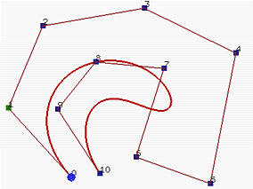
This nice property allows us to design very complicated shapes with lower degree polynomials. For example, the right figure below shows a Bézier curve with the same set of control points. It still cannot follow the control polygon nicely even though its degree is 10!
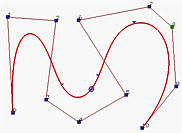
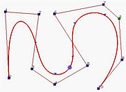
In general, the lower the degree, the closer a B-spline curve follows its control polyline. The following figures all use the same control polyline and knots are clamped and uniformly spaced. The first figure has degree 7, the middle one has degree 5 and the right figure has degree 3. Therefore, as the degree decreases, the generated B-spline moves closer to its control polyline.
Since each control point needs a basis function and the number of basis functions satisfies m = n + p + 1.
Note that basis function N0,p(u) is the coefficient of control point p0 and is non-zero on [u0,up+1). Since u0 = u1 = ... = up = 0 for a clamped B-spline curve, N0,0(u), N1,0(u), ...., Np-1,0(u) are zero and only Np,0(u) is non-zero (recall from the triangular computation scheme). Consequently, when u = 0, N0,p(0) is 1 and p(0) = p0. A similar discussion can show p(1) = pn
If u is in knot span [ui, ui+1), there are only p+1 basis functions (i.e., Ni,p(u), ... , Ni-p+1,p(u), Ni-p,p(u)) non-zero on this knot span. Since Nk,p(u) is the coefficient of control point pk, only p+1 control points pi, pi-1, pi-2, .., pi-p have non-zero coefficients. Since on this knot span the basis functions are non-zero and sum to 1, their "weighted" average, p(u), must lie in the convex hull defined by control points pi, pi-1, pi-2, .., pi-p. The meaning of "strong" is that while p(u) still lies in the convex hull defined by all control points, it lies in a much smaller one.
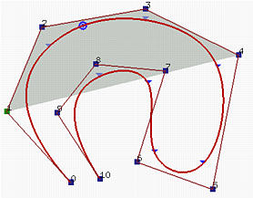
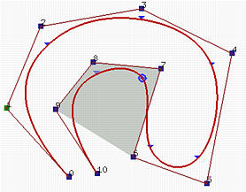
The above two B-spline curves have 11 control points (i.e., n = 10), degree 3 (i.e., p=3) and 15 knots (m = 14) with first four and last four knots clamped. Therefore, the number of knot spans is equal to the number curve segments. The knot vector is
| u0 | u1 | u2 | u3 | u4 | u5 | u6 | u7 | u8 | u9 | u10 | u11 | u12 | u13 | u14 |
| 0 | 0 | 0 | 0 | 0.12 | 0.25 | 0.37 | 0.5 | 0.62 | 0.75 | 0.87 | 1 | 1 | 1 | 1 |
The left figure has u in knot span [u4, u5) = [0.12,0.25) and the corresponding point (i.e. p(u)) in the second curve segment. Therefore, there are p+1 = 4 basis functions non-zero on this knot span (i.e., N4,3(u), N3,3(u), N2,3(u) and N1,3(u) ) and the corresponding control points are p4, p3, p2 and p1. The shaded area is the convex hull defined by these four points. It is clear that p(u) lies in this convex hull.
The B-spline curve in the right figure is defined the same way. However, u is in [u9, u10) = [0.75,0.87) and the non-zero basis functions are N9,3(u), N8,3(u), N7,3(u) and N6,3(u). The corresponding control points are p9, p8, p7 and p6.
Consequently, as u moves from 0 to 1 and crosses a knot, a basis functions becomes zero and a new non-zero basis function becomes effective. As a result, one control point whose coefficient becomes zero will leave the the definition of the current convex hull and is replaced with a new control point whose coefficient becomes non-zero.
This follows from another important property of B-spline basis functions. Recall that Ni,p(u) is non-zero on interval [ui, ui+p+1). If u is not in this interval, Ni,p(u)pi has no effect in computing p(u) since Ni,p(u) is zero. On the other hand, if u is in the indicated interval, Ni,p(u) is non-zero. If pi changes its position, Ni,p(u)pi is changed and consequently p(u) is changed.
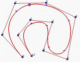
The above B-splines are defined with the same parameters as in the previous convex hull example. We intent to move control point p2. The coefficient of this control point is N2,3(u) and the interval on which this coefficient is non-zero is [u2, u2+3+1) = [u2, u6) = [0,0.37). Since u2 = u3 = 0, only three segments that corresponds to [u3, u4) (the domain of the first curve segment), [u4, u5) (the domain of the second curve segment) and [u5, u6) (the domain of the third curve segment) will be affected. The right figure shows the result of moving p2 to the lower right corner. As you can see, only the first, second and third curve segments change their shapes and all remaining curve segments stay in their original place without any change.
This local modification scheme is very important to curve design, because we can modify a curve locally without changing the shape in a global way. Moreover, if fine-tuning curve shape is required, one can insert more knots (and therefore more control points) so that the affected area could be restricted to a very narrow region. We shall talk about knot insertion later.
If u is not a knot, p(u) is in the middle of a curve segment of degree p and is therefore infinitely differentiable. If u is a knot in the non-zero domain of Ni,p(u), since the latter is only Cp-k continuous, so does p(u).
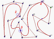
The above B-spline curve has 18 control points (i.e., n = 17), degree 4 and the following clamped knot vector
| u0 to u4 | u5 | u6 and u7 | u8 | u9 to u11 | u12 | u13 to u16 | u17 | u18 to u22 |
| 0 | 0.125 | 0.25 | 0.375 | 0.5 | 0.625 | 0.75 | 0.875 | 1 |
Thus, u6 is a double knot, u9 is a triple knot and u13 is a quadruple knot. Consequently, p(u) is of C4 continuous at any point that is not a knot, C3 continuous at all simple knots, C2 continuous at u6, C1 continuous at u9, C0 continuous at u13.
All points on the curve that correspond to knots are marked with little triangles. Those corresponding to multiple knots are further marked with circles and their multiplicities. It is very difficult to visualize the difference between C4, C 3 and even C2 continuity. For the C1 case, the the corresponding point lies on a leg, while the C0 case forces the curve to pass through a control point. We shall return to this issue later when discussing modifying knots.
The variation diminishing property also holds for B-spline curves. If the curve is in a plane (resp., space), this means no straight line (resp., plane) intersects a B-spline curve more times than it intersects the curve's control polyline.
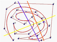
In the above figure, the blue line intersects both the control polyline and the B-spline curve 6 times, while the yellow line also intersects the control polyline and the B-spline curve 5 times. However, the orange line intersects the control polyline 6 times and the curve 4 times.
If n = p (i.e., the degree of a B-spline curve is equal to n, the number of control points minus 1), and there are 2(p + 1) = 2(n + 1) knots with p + 1 of them clamped at each end, this B-spline curve reduces to a Bézier curve.
The affine invariance property also holds for B-spline curves. If an affine transformation is applied to a B-spline curve, the result can be constructed from the affine images of its control points. This is a nice property. When we want to apply a geometric or even affine transformation to a B-spline curve, this property states that we can apply the transformation to control points, which is quite easy, and once the transformed control points are obtained the transformed B-spline curve is the one defined by these new points. Therefore, we do not have to transform the curve.

