Notes
on obtaining empirical heat of mixing curve:
( For this part of the project, click here
for a sample template.)
-
Input the raw data.
-
Exclude the missing data. (For example, in Appendix B-11, for r=20,
there is no entry for
 ,
so there is no need to include it as part of the raw data.)
,
so there is no need to include it as part of the raw data.)
-
Just use a large number for r = infinity. (For example, use r =
107 ).
-
Include an extra data point for approximately pure H2SO4.
(For example, for r = 10-3, enter =
0)
-
Create a column for the estimates based on your model.
-
Create a column for the square of the errors between data and estimates.
-
Create a cell for the RMS (root mean of squared errors ).
-
Minimize the RMS by using SOLVER to change the parameters.
-
Generate another table to observe how close the model fits the data.
-
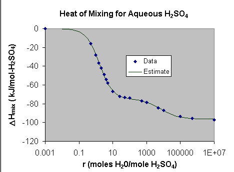
Because of the particular behavior of heats of mixing around the dilution,
it is advisable to plot
as a function of r with the r-axis in logarithm scale.
-
To generate the model curve, create a column that varies linearly from
say n=-2 to 7. Next, generate the r values via a formula such as
r = 10^n. Using the model parameters obtained from step 5, you could
now generate the corresponding specific heats of mixing.
-
Now plot the model curve and the raw data in the same graph to observe
how close the model fits the data.
( To change the axis to logarithmic scale, first right-click on the axis
and select FORMAT AXIS. A window should appear.
 Under the SCALE tab, check the selection LOGARITHMIC SCALE.)
For this particular mixing process you should obtain a model that matches
the data pretty closely as shown in the figure below.
This page is maintained by Tomas B. Co (tbco@mtu.edu). Last
revised 4/20/2000.
Tomas B. Co
Associate Professor
Department of Chemical Engineering
Michigan Technological University
1400 Townsend Avenue
Houghton, MI 49931-1295
Back to Homepage