Given: a differential equation

Required: a series of number-pairs,
(t0,x0) , (t1,x1) , (t2,x2) , , (tN,xN)
(For a pdf
version, click here)
I. Euler Method for Solving Initial Value Problems

Required: a series of number-pairs,
(t0,x0) , (t1,x1) , (t2,x2) , , (tN,xN)
dx/dt »Dx/Dt
where Dx = xk+1 -
xk
dx/dt »Dx/Dt = f(tk,xk,uk)
xk+1-xk=Dt f(tk,xk,uk)
xk+1=xk+Dt f(tk,xk,uk)
where we have set the evaluation of the function f at t=tk, and so uk is just u(t=tk).
The last equation above is known as the recursion equation,
also known as the finite difference approximation. All terms on the left-hand
side of the recursion equation are known (current values used). Evaluating
the left-hand side yields (predicts) the next value of x in the series.
x1 = x0 + Dt f(0,x0,u0)
x3 = x2 + Dt f( 2Dt, x2, u2 )
xN = xN-1 + Dt f( (N-1)Dt, xN-1, uN-1)
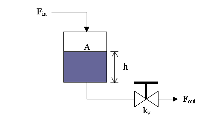
The main purpose of a simulation is to observe changes
in the behavior when certain parameters of the system are tweaked.
For our scenario, let us choose the following settings:
Fin=1 ft3/sec
kv=1.25 ft2.5
A=0.75 ft2
and we will treat kv and A as parameters. For our initial condition, let h(0)=1 ft.
To compare our case with the discussion of Eulers method above, we have x=h , u=Fin , and
f( t, x, u )=f( t, h, Fin )=( Fin - kvh1/2 ) /A
so the recursion equation is given by
hk+1 = hk + Dt ( Fin,k - kvhk1/2 )/A
Now, let us implement this in a spreadsheet (figures below were generated using Microsoft Excel):
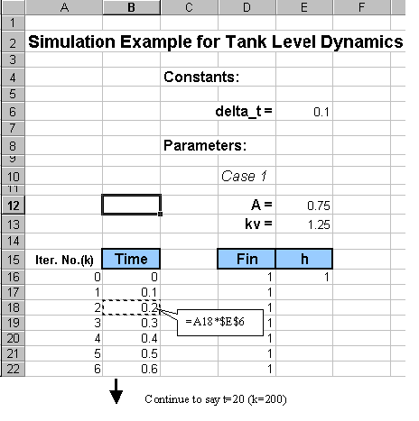
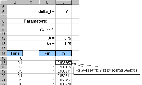
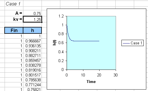
4. As mentioned earlier, to investigate how the response
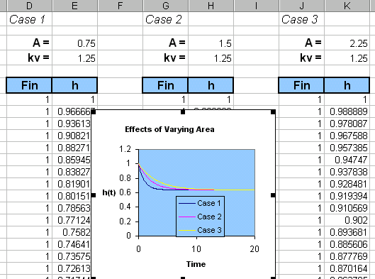
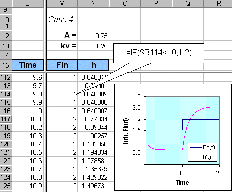
will behave to a set of parameter changes, we can collect several cases
by copying the block from cell D10 to E216 to another location and then
change one of the parameters, say A below:
III. Higher Order Differential Equations

We first need to introduce new variables to denote the derivatives. Let v = dx/dt, then we can reduce the original second order equation to a set of 2 first order equations given by
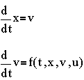
Following the same approach as before of approximating derivatives by finite differences, we get two recursion equations
xk+1 = xk + Dt vk
vk+1 = vk + Dt f(tk,xk,vk,uk)
The simulation will be initialized by conditions x0=x(0)
and v0= dx/dt(0).
This page is maintained by Tomas B. Co (tbco@mtu.edu). Last revised 12/2/98.
Tomas B. Co
Associate Professor
Department of Chemical Engineering
Michigan Technological University
1400 Townsend Avenue
Houghton, MI 49931-1295