Introductory R Tutorial 1: Basics
Shane T. Mueller shanem@mtu.edu
Michigan Technological University
Shane T. Mueller shanem@mtu.edu
Michigan Technological University
Return to main site | Lesson 1 | Lesson 2 | Lesson 3 | Lesson 4 | Lesson 5
Download Lesson 1 files here
You can share annotations, questions, and answers on any of these pages using hypothes.is. Use this link to join the group
The goals of the first session are to familiarize you with R and R studio. After installing these separate systems, you will learn:
R Studio is created by a company that has created a professional frontend for R. They license the R studio with an open-source license, but also sell support and several server and other things that some people pay for. It has become one of the most important popularizers of R, and the default front-end that most people use.
You will probably need to download R and R studio separately. You can download R from our local MTU server:
And download R studio from the R studio page:
https://rstudio.com/products/rstudio/download/
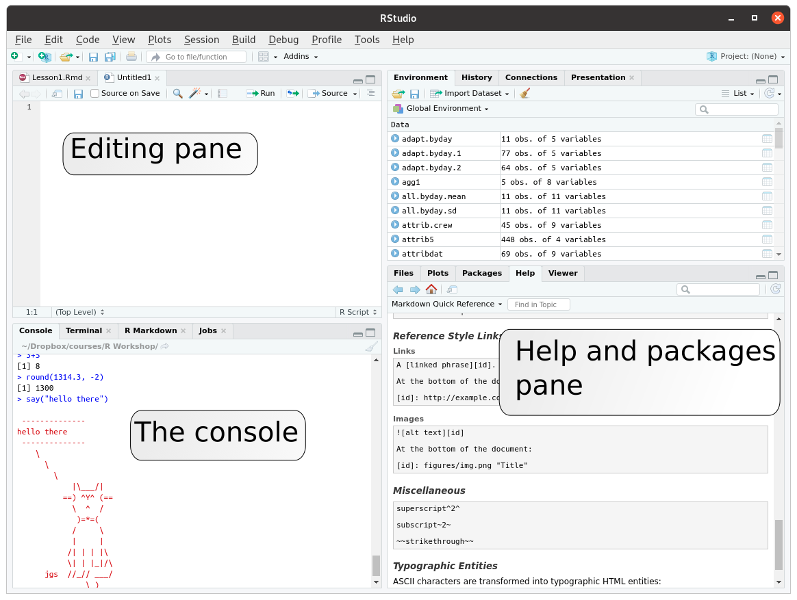
When you load R studio, it will look something like this. There are four panels or panes. Today, we will focus on three: the editing pane, the console pane, and the help/packages pane.

Screenshot of R studio
At the bottom left of the screen is the console, where the ‘R’ interpreter lives. It is basically a calculator. Try typing in an expression like 3+5 at the ‘>’ prompt (don’t type the ‘>’ symbol):
> 3+5
[1] 8
You can see that the expression evaluates to 8, and that value is printed in the console. We say that the expression evaluates to or returns the value of 8, because that value can be used by something else, including a more complex expression. The [1] indicates that a single number is returned, and you can safely ignore that for now. Everything you do will be executed by an interpreter, often the one in this console, but sometimes one running behind the scenes. You can run the R interpreter without using R studio. It can be run on web servers to make dynamic web analytics. It runs inside other graphical analysis programs like JASP and JAMOVI. You can type commands into the console, or have it read and process files to run a series of commands. The web page you are currently looking was made by an R interpreter working behind the scenes to process a file. Unlike many statistical programs for which a data table is the central focus, in R the console and its interpreter is.
Try to do the following and determine what happens:
3+(4*5) versus (3+4)*5. Pay attention to how R inserts the closing parenthesis automatically.3+ 4 +. Try to complete the expression after you hit enter.At its core, R is a complex calculator called an interpreter. You can use it to do complex operations on data, but it works, at its core, very much like your pocket calculator.
R also has functions that will do more complex operations. A function has a name, and it is called by writing the name of the function followed by (), and an expression can usually be put inside the parentheses. One useful function is round(), and you can use it like this:
> round(3.36)
[1] 3
Functions have multiple arguments, these arguments have both an order and names. Furthermore, many of the arguments have default values. If you type the name of the function in the console, you can see its definition, and especially the arguments it takes:
> round
function (x, digits = 0)  .Primitive("round")
This shows that the round function takes two arguments. The first is called ‘x’, and the second is called ‘digits’. Digits has a default value of 0, so when we used round previously, it used a digits value of 0, which is why it rounded to the nearest digit. In R, if a function is called with arguments without names, it binds them in the order they are applied. So, if I type the following, it knows the first number is bound to ‘x’ and the second number is bound to ‘digits’:
> round(13.3245,1)
[1] 13.3
We cannot call round without an x value, but we can call round with named arguments instead of using the default slots. When doing this, we can call them in any order we want, or start naming non-default arguments after we provide the default ones. And the first default argument will be bound to the first un-named value given. Notice that when naming arguments, R will be satisfied with partial matching; if you get the first characters of an argument right, and it is enough to distinguish it from other arguments, it will succeed
Here are some examples to try:
> round(digits=3,x=3145.1)
[1] 3145.1
> round(393.313414,digits=-2)
[1] 400
> round(digits=3,3145.1)
[1] 3145.1
>  round(x=3552.5252, d =-1)
[1] 3550
R functions will also fail when used incorrectly. This is usually to help you get the right results; if instead of failing they tried to guess what you wanted, you would never know if the guess was wrong. This sometimes includes checking for missing values, arguments used multiple times, giving the wrong number of arguments, and giving the wrong type of argument.
Try each of the following. Identify what you think will happen before you enter the command, and see if you are right. Some of these will produce errors. If an error is produced, explain why the error occurred.
hello() by typing it into the console.Try running each of the following. Before each one, predict what should happen and whether it will lead to an error. Some of these look like dumb mistakes, but they will all happen if you use R.
round(13.5, 3, 9)round(13.12515,2,x=5)round(13.12515,digit=3,digits=1)round(x=12.22,x=15.33)round("hello",3)round(digits=5)
Functions are very powerful, and we will later learn how to make them ourselves, which will help you repeat complex operations without copy/pasting, and to generalize analyses so you can apply them to multiple data sets. For now, it is enough to know how to use them.
In the upper left of the screen is an editor, and you might even have this file open in it. You can have a number of documents open in different tabs. We will focus on two types of documents you might use.
We will deal with markdown at the end of this lesson. For now, we want to create an .R file and enter some calculations and expressions in the file.
When you enter different expressions into an R script file, you can run the entire file, or parts of the file by selecting the region you want to run. This is helpful in debugging or testing. It is a good practice to work within an .R file instead of the console, so you always have a record of what you are doing.
Any line that starts with # is ignored in the console and the script file. And anything that follows the # on a line. You can use this to make comments to help you remember what you have entered.
Even before you save the file, you can execute a line by selecting it and hitting -> run, or selecting a region and hitting ctrl-enter. There are actually many ways of sending code to the console though–look at the Code menu under the Run section for some other options. You can also use ctrl-shift-enter for running the entire file. source() loads the file in the background.
It is important to be systematic about saving what you are doing so it can be redone later. You should always aim to be able to completely re-run the steps you take to accomplish something based on a series of commands saved in your file. Because you can work simultaneously in the console and a .R file, it is a common mistake to do something in the console, or mix up the order of something in your file, and then when you return to it later, it will not work. You should also start developing good habits about how you save and name these files, separate them from data, and document what you are doing in the files using # comments. You will thank yourself later when you can return to an analysis you did in the past and be able to jump in and know what is going on.

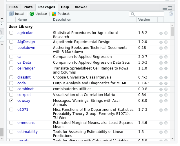
R Studio packages pane
One of the advantages of R is that it gives you access to thousands of special-purpose packages that help you do specific analyses. There are many advanced techniques that are available first as R packages, or only as R packages, and the commercial packages are lagging or lacking.
The built-in or installed packages you have are avialable in the ‘Packages’ tab on the lower right. There are websites that list many of them, but if you know the name of the package, you can hit the ‘install’ button, enter the name, and it will download and install for you. You can also run the function install.packages(), giving it the text name of the package you want to install.
We will try to install the ‘fortunes’ package. Try typing fortunes into the packages|install entry, or enter the following into the console, which should produce the following output:
install.packages("fortunes")

Installing package into ‘/home/smueller/R/x86_64-pc-linux-gnu-library/3.6’
(as ‘lib’ is unspecified)
trying URL 'https://cloud.r-project.org/src/contrib/fortunes_1.5-4.tar.gz'
Content type 'application/x-gzip' length 192938 bytes (188 KB)
==================================================
downloaded 188 KB

* installing *source* package ‘fortunes’ ...
** package ‘fortunes’ successfully unpacked and MD5 sums checked
** using staged installation
** R
** inst
** byte-compile and prepare package for lazy loading
** help
*** installing help indices
** building package indices
** installing vignettes
** testing if installed package can be loaded from temporary location
** testing if installed package can be loaded from final location
** testing if installed package keeps a record of temporary installation path
* DONE (fortunes)

The downloaded source packages are in
    ‘/tmp/RtmpxuCwVJ/downloaded_packages’
You can download as many packages as you want, but they will not be accessible to you until you load them. If you look through the packages pane for ‘fortunes’ you will see that it does not have a checkmark beside it. If you click on the checkmark, you will see that the text library(fortunes) appears in the console. Instead of clicking the checkmark, you could alternately type this into the console, or put it at the top of your .R file.
The R packages system are one of the most powerful and exciting parts of R. It is one of the things that truly separates it from most competition. For almost any analysis or statistic you want to perform, there are likely to be one or more packages out there that do what you want. The trick is figuring out how to use them, which is why we rely on the help system.

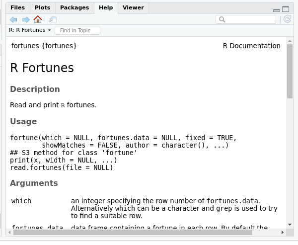
R Studio help pane
We have loaded two libraries, but we have no idea what they do or how to use them. Luckily, there is extensive help within R. Navigate to the fortunes line in the packages tab, and click on the blue link to get help. Alternately, you can type ?fortunes or help(fortunes). These will open up the help file in the help tab. If we do that, the documentation below is displayed in the help panel for the library, which looks like this. This tells us all the functions that the library provides:
Documentation for package ‘fortunes’ version 1.5-4
DESCRIPTION file.
User guides, package vignettes and other documentation.

Help Pages
fortune             R Fortunes
fortunes              R Fortunes
print.fortune         R Fortunes
read.fortunes         R Fortunes
toLatex.fortune     R Fortunes
If you click on fortune or type help(fortune), it will send you to a specific help file for that function:
help(fortune)

R Fortunes
Description
Read and print R fortunes.

Usage
fortune(which = NULL, fortunes.data = NULL, fixed = TRUE,
        showMatches = FALSE, author = character(), ...)
## S3 method for class 'fortune'
print(x, width = NULL, ...)
read.fortunes(file = NULL)
The help gives more details about the arguments and the value (what is returned from the function.) We can see that fortunes provides a function called fortune(), and the fortune() function takes a number of arguments, although none are are needed. The =NULL tells us that the default value is NULL, and so it is really not needed. This should give you all the information you need to run a library function. Usually, examples are also provided in the help file.
Sometimes when you search for a function help using ? or ??, you will get to a page within the library but not the one you want. You can usually scroll to the bottom of that help page to find an ‘index’ link which will take you to the main help for a package.
If you don’t know how to use a function, or it does not seem to be working as expected, the first place to look is the help. This sounds obvious, but I have learned that it is not always. When using a new library, I often have to pause in the middle of an analysis, work through some examples in the help in order to test how the function works, and then return to the analysis more confident in how to apply the function I am interested in.
We looked at creating .R files earlier. The web page you are probably reading is generated from another kind of file, called a markdown file. It is similar to an R file but has an extension of .Rmd. Open the Lesson1.Rmd file and see what it looks like.
R Markdown files must end in the Rmd extension, and start with some header information that looks like this:
---
title: "Introductory R Tutorial 1: Basics"
author: Shane Mueller
date: July 4, 1776
output:
  word_document:
---
I have a lot more options in the current file to allow me to make the special html page and pdfs, and auto-date the document. Following this header, you can add formatted text using simple markdown code–which is how I have used this so far. Using the ‘knit’ button, you can choose how you want the markdown formatted–without installing additional packages, you probably can knit to a .docx file or a plain .html file, but .pdf and fancier .html are also possible.
There are detailed tutorials in using markdown to format text, and for basic support, just go to the Help|R Markdown Quick Reference and some markdown examples are shown in the help pane.
However, more interesting is that you can embed R code in a markdown file, and it will run the code and display the output to the generated file. You specify it with the following pattern:

Example markdown used in this document
We can see that in the following code block, the code and the results of each line are printed in the final document.
## [1] 3## [1] 8## [1] 1300##
## --------------
## hello there
## --------------
## \
## \
## \
## |\___/|
## ==) ^Y^ (==
## \ ^ /
## )=*=(
## / \
## | |
## /| | | |\
## \| | |_|/\
## jgs //_// ___/
## \_)
## Within R, you can hit the green ‘play’ button for any code block and see the result. You will need to load any library in document if you plan on using it, even if you have loaded in in your console, because the markdown creates a fresh R instance to generate the document.
Create your own new markdown file from the File|New File| R Markdown menu. Consult the quick reference for more guidance. Some things to try:
Make a block of code and enter some calculations or functions into a code block.
At each step, knit the file into a word document and open that document to see your progress and to be sure you have not made any errors.
Using markdown is very powerful, and gives the ability to document what you are doing, create reports, and also create the basis for a report that easily gets edited to a shorter version you may give a client.
The concepts we learned today cover how to use the basic aspects of R. You will use most of these all the time, and so most tutorials forget to explain these basics to new users.